pytorch computation graph

1. 动态图 vs 静态图

pytorch 是动态建图，好处是方便使用python control flow statements控制计算流走向，每个iteration可以有完全不同的计算图，同时也比较容易处理shape不确定的tensors or variables。除此，dynamic graphs are debug friendly, becuase it allows for line by line execution of code and you can have access to all variables and tensors.

tensorflow 是静态图，先建图后计算，而且一旦建图完成，graph就不能再改变，只能通过feeding和fetch来决定运行哪个subgraph， 需要在建图时考虑所有需要的计算结构。而且，也不方便调试。好处是不需要动态建图，速度快些。

2. graph creation 和 freeing 

每个iteration，in forward pass 计算图都重头重新创建一次。 创建计算图是为了自动求导 in backward pass, 所以如果没有需要计算梯度的变量存在，那么在前馈通路中，计算图不会也不需要创建， 如inference mode 下。 

计算图是在forward时通过迭代的tracing tensors or variables that require gradients 来创建的，不是在loss.backward()时根据实际需要创建的。

In forward pass, 在计算图上的intermediate nodes的前馈结果会被分配空间暂存到buffers，用于backward时计算梯度。 一旦梯度计算完成，计算图和buffers会被释放，来节约内存。所以，同一个计算图，backward两次是会报错的。

example 1 

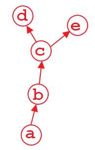
Suppose that we have a computation graph shown above. The variable d and e is the output, and a is the input. For example,

import torch
from torch.autograd import Variable
a = Variable(torch.rand(1, 4), requires_grad=True)
b = a**2
c = b*2
d = c.mean()
e = c.sum()

when we do d.backward(), that is fine. After this computation, the part of graph that calculate d will be freed by default to save memory. So if we do e.backward(), the error message will pop up. In order to do e.backward(), we have to set the parameter retain_graph to True in d.backward(), i.e.,

d.backward(retain_graph=True)

As long as you use retain_graph=True in your backward method, you can do backward any time you want:

d.backward(retain_graph=True) # fine
e.backward(retain_graph=True) # fine
d.backward() # also fine
e.backward() # error will occur!

example 2

                    -- FC - FC - FC - cat?
Conv - Conv - Conv -|
                    -- FC - FC - FC - car?

Given a picture that we want to run both branches on, when training the network, we can do so in several ways. First , we simply compute a loss on both assessments and sum the loss, and then backpropagate.

However, there’s another scenario – in which we want to do this sequentially. First we want to backprop through one branch, and then through the other. In that case, running .backward() on one graph will destroy any gradient information in the convolutional layers, too, and the second branch’s convolutional computations  will not contain a complete graph anymore (Conv-Conv-Conv have been freed) ! That means, that when we try to backprop through the second branch, Pytorch will throw an error since it cannot find a graph connecting the input to the output! In these cases, we can solve the problem by simple retaining the graph on the first backward pass. The graph will then not be consumed, but only be consumed by the first backward pass that does not require to retain it.

今天的文章pytorch computation graph分享到此就结束了，感谢您的阅读，如果确实帮到您，您可以动动手指转发给其他人。