本博客与以下文档资料一起服用效果更佳。
Matlab源码地址:
开始正文。
梳理一下本篇博客图像拼接的原理:
- 特征检测:SIFT角点检测
- 特征描述:SIFT描述子
- 特征匹配:暴力搜索+欧氏距离
- 求变换矩阵:最小二乘法+RANSAC+仿射变换
- 拼接多幅图像
完整实现一个SIFT都很麻烦,也并没必要。本博客是在斯坦福大学计算机视觉课程大作业的基础上实现的,读者也可以按课程PPT及作业pdf指导书,自己实现一遍,定会加深自己对其中关键算法的理解。
本博客根据其作业指导书,展示其中一些算法的Matlab代码实现。
<译>
#1.引文
全景拼接是计算机视觉领域取得的一项早期成就。在2007年,Brown 和 Lowe发表了著名的图像拼接论文。自打那以后,自动全景拼接技术受到广泛应用,例如Google街景地图、智能手机上的全景照片、拼接软件比如Photosynth和AutoStitch。
在这个大作业中,我们会从多幅图像中匹配SIFT关键点,来构建单幅全景图片。这涉及以下任务:
使用高斯差分(DoG)检测器找关键点,返回它的坐标位置和尺度。(这一步已经提供给你)
给一副图像的每个关键点构建SIFT描述子。
从两幅不同的图像中比较两组SIFT描述子,找到匹配点。
给定一个关键点匹配的列表,使用最小二乘法找到仿射变换矩阵,这个矩阵能将iamge1上的位置映射到image2上的位置。
使用RANSAC使仿射变换矩阵的估计具有更好的鲁棒性。
给定变换矩阵,使用它变换(平移、尺度、或者倾斜)image1,将它覆盖到image2上面,构建一个全景图。(这一步已经提供给你)
在真实世界场景中的特定例子中,把多幅图像拼接在一起。
<译>
#2.构建SIFT描述子
复习SIFT算法的讲义PPT,编写给定的SIFTDescriptor.m,来为每个DoG关键点,产生SIFT关键点描述子。注意关键点的位置和尺度已经提供给你,使用的是高斯金字塔。
运行提供的EvaluateSIFTDescriptor.m,检查你的实现。
这一步需要自己写的代码包括计算图像导数(x和y方向)、梯度(大小和方向)、计算邻域块的主方向、每个采样点的梯度相对方向、计算直方图的变量(方向箱子的划分,每个箱子的幅值)、计算梯度直方图以及将其串接进一个1*128的数组中。
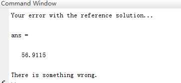
代码提供了标准的结果数据和测试代码,经过测试,我编写的SIFT与标准数据偏差明显。
注:感谢yuanyuan12222的评论指正。出现偏差的原因是:主方向选取没有向下取(308行注释有说明),将312行代码direction =2piloc(1)/num_bins;改为direction =2pi(loc(1)-1)/num_bins;就OK了。
说明我的某部分实现不符合标准实现。但由最后的拼接效果来看,实现是可用的。
我的实现(Matlab代码):
SIFTDescriptor.m
function descriptors = SIFTDescriptor(pyramid, keyPtLoc, keyPtScale)

% SIFTDescriptor Build SIFT descriptors from image at detected key points'
% location with detected key points' scale and angle
%
% INPUT:
%   pyramid: Image pyramid. pyramid{i} is a rescaled version of the
%            original image, in grayscale double format
%
%   keyPtLoc: N * 2 matrix, each row is a key point pixel location in
%   pyramid{round(keyPtScale)}. So pyramid{round(keyPtScale)}(y,x) is the center of the keypoint
%
%   keyPtScale: N * 1 matrix, each entry holds the index in the Gaussian
%   pyramid for the keypoint. Earlier code interpolates things, so this is a
%   double, but we'll just round it to an integer.
%
% OUTPUT:
%   descriptors: N * 128 matrix, each row is a feature descriptor
%

    % Precompute the gradients at all pixels of all pyramid scales

    % This is a cell array, which is like an ArrayList that holds matrices.
    % You use {} to index into it, like this: magnitude = grad_mag{1}
    grad_theta = cell(length(pyramid),1);
    grad_mag = cell(length(pyramid),1);

    for scale = 1:length(pyramid)
        currentImage = pyramid{scale};
%%%%%%%%%%%%%%%%%%%%%%%%%%%%%%%%%%%%%%%%%%%%%%%%%%%%%%%%%%%%%%%%%%%%%%%%%%%%%%%%
%                                                                              %
%                                YOUR CODE HERE                                %
%                          Read the doc for filter2.                           %
%                Use with the filter [-1 0 1] to fill in img_dx,               %
%                  and the filter [-1;0;1] to fill in img_dy.                  %
%                    Please use the filter2 'same' option so                   %
%                the result will be the same size as the image.                %
%                                                                              %
%%%%%%%%%%%%%%%%%%%%%%%%%%%%%%%%%%%%%%%%%%%%%%%%%%%%%%%%%%%%%%%%%%%%%%%%%%%%%%%%
        % gradient image, for gradients in x direction.
        img_dx = zeros(size(currentImage));
        img_dx=filter2([-1 0 1],currentImage);
        % gradients in y direction.
        img_dy = zeros(size(currentImage));
        img_dy=filter2([-1;0;1],currentImage);

%%%%%%%%%%%%%%%%%%%%%%%%%%%%%%%%%%%%%%%%%%%%%%%%%%%%%%%%%%%%%%%%%%%%%%%%%%%%%%%%
%                                                                              %
%                               END OF YOUR CODE                               %
%                                                                              %
%%%%%%%%%%%%%%%%%%%%%%%%%%%%%%%%%%%%%%%%%%%%%%%%%%%%%%%%%%%%%%%%%%%%%%%%%%%%%%%%


%%%%%%%%%%%%%%%%%%%%%%%%%%%%%%%%%%%%%%%%%%%%%%%%%%%%%%%%%%%%%%%%%%%%%%%%%%%%%%%%
%                                                                              %
%                                YOUR CODE HERE                                %
%                Use img_dx and img_dy to compute the magnitude                %
%                   and angle of the gradient at each pixel.                   %
%       store them in grad_mag{scale} and grad_theta{scale} respectively.      %
%           The atan2 function will be helpful for calculating angle           %
%                                                                              %
%%%%%%%%%%%%%%%%%%%%%%%%%%%%%%%%%%%%%%%%%%%%%%%%%%%%%%%%%%%%%%%%%%%%%%%%%%%%%%%%
         % Calculate the magnitude and orientation of the gradient.
        grad_mag{scale} = zeros(size(currentImage));
        grad_theta{scale} = zeros(size(currentImage));
        grad_mag{scale}=sqrt(img_dx.^2+img_dy.^2);
        grad_theta{scale}=atan2(img_dy,img_dx);


%%%%%%%%%%%%%%%%%%%%%%%%%%%%%%%%%%%%%%%%%%%%%%%%%%%%%%%%%%%%%%%%%%%%%%%%%%%%%%%%
%                                                                              %
%                               END OF YOUR CODE                               %
%                                                                              %
%%%%%%%%%%%%%%%%%%%%%%%%%%%%%%%%%%%%%%%%%%%%%%%%%%%%%%%%%%%%%%%%%%%%%%%%%%%%%%%%
        % atan2 gives angles from -pi to pi. To make the histogram code
        % easier, we'll change that to 0 to 2*pi.
        grad_theta{scale} = mod(grad_theta{scale}, 2*pi);

    end

    % The number of bins into which each gradient vector will be placed.
    num_angles = 8;

    % The patch extracted around each keypoint will be divided into a grid
    % of num_histograms x num_histograms.
    num_histograms = 4;

    % Each histogram covers an area "pixelsPerHistogram" wide and tall
    pixelsPerHistogram = 4;

    % For each keypoint we will extract a region of size
    % patch_size x patch_size centered at the keypoint.
    patch_size = num_histograms * pixelsPerHistogram;

    % Number of keypoints that were found by the DoG blob detector
    N = size(keyPtLoc, 1);

    % Initialize descriptors to zero
    descriptors = zeros(N, num_histograms * num_histograms * num_angles);

    % Iterate over all keypoints
    for i = 1 : N

        scale = round(keyPtScale(i));
        % Find the window of pixels that contributes to the descriptor for the
        % current keypoint.
        xAtScale = keyPtLoc(i, 1);%center of the DoG keypoint in the pyramid{2} image
        yAtScale = keyPtLoc(i, 2);
        x_lo = round(xAtScale - patch_size / 2);
        x_hi = x_lo+patch_size-1;
        y_lo = round(yAtScale - patch_size / 2);
        y_hi = y_lo+patch_size-1;


        % These are the gradient magnitude and angle images from the
        % correct scale level. You computed these above.
        magnitudes = grad_mag{scale};
        thetas = grad_theta{scale};
        try
            % Extract the patch from that window around the keypoint
            patch_mag = zeros(patch_size,patch_size);
            patch_theta = zeros(patch_size,patch_size);
            patch_mag = magnitudes(y_lo:y_hi,x_lo:x_hi);
            patch_theta = thetas(y_lo:y_hi,x_lo:x_hi);
        catch err
            % If any keypoint is too close to the boundary of the image
            % then we just skip it.
            continue;
        end

%%%%%%%%%%%%%%%%%%%%%%%%%%%%%%%%%%%%%%%%%%%%%%%%%%%%%%%%%%%%%%%%%%%%%%%%%%%%%%%%
%                                                                              %
%                              YOUR CODE HERE:                                 %
%                                                                              %
%  Express gradient directions relative to the dominant gradient direction     %
%                              of this keypoint.                               %
%                                                                              %
%            HINT: Use the ComputeDominantDirection function below.            %
%                                                                              %
%%%%%%%%%%%%%%%%%%%%%%%%%%%%%%%%%%%%%%%%%%%%%%%%%%%%%%%%%%%%%%%%%%%%%%%%%%%%%%%%
        % Step 1: compute the dominant gradient direction of the patch
        patch_angle_offset = ComputeDominantDirection(patch_mag, patch_theta);
        % Step 2: change patch_theta so it's relative to the dominant direction
        patch_theta = patch_theta-patch_angle_offset;


%%%%%%%%%%%%%%%%%%%%%%%%%%%%%%%%%%%%%%%%%%%%%%%%%%%%%%%%%%%%%%%%%%%%%%%%%%%%%%%%
%                                                                              %
%                              END OF YOUR CODE                                %
%                                                                              %
%%%%%%%%%%%%%%%%%%%%%%%%%%%%%%%%%%%%%%%%%%%%%%%%%%%%%%%%%%%%%%%%%%%%%%%%%%%%%%%%

        % This line will re-map patch_theta into the range 0 to 2*pi
        patch_theta = mod(patch_theta, 2*pi);
        % Weight the gradient magnitudes using a gaussian function
        patch_mag = patch_mag .* fspecial('gaussian', patch_size, patch_size / 2);


%%%%%%%%%%%%%%%%%%%%%%%%%%%%%%%%%%%%%%%%%%%%%%%%%%%%%%%%%%%%%%%%%%%%%%%%%%%%%%%%
%                                                                              %
%                             YOUR CODE HERE:                                  %
%                                                                              %
%         Compute the gradient histograms and concatenate them in the          %
%  feature variable to form a size 1x128 SIFT descriptor for this keypoint.    %
%                                                                              %
%            HINT: Use the ComputeGradientHistogram function below.            %
%                                                                              %
%%%%%%%%%%%%%%%%%%%%%%%%%%%%%%%%%%%%%%%%%%%%%%%%%%%%%%%%%%%%%%%%%%%%%%%%%%%%%%%%
        % The patch we have extracted should be subdivided into
        % num_histograms x num_histograms cells, each of which is size
        % pixelsPerHistogram x pixelsPerHistogram.

        % Compute a gradient histogram for each cell, and concatenate
        % the histograms into a single feature vector of length 128.

        % Please traverse the patch row by row, starting in the top left,
        % in order to match the given solution. E.g. if you use two
        % nested 'for' loops, the loop over x should  be the inner loop.

        % (Note: Unlike the SIFT paper, we will not smooth a gradient across
        % nearby histograms. For simplicity, we will just assign all
        % gradient pixels within a pixelsPerHistogram x pixelsPerHistogram
        % square to the same histogram.)

        % Initializing the feature vector to size 0. Hint: you can
        % concatenate the histogram descriptors to it like this:
        % feature = [feature, histogram]
        feature = [];
        subdivided_patch_theta=zeros(pixelsPerHistogram,pixelsPerHistogram);
        subdivided_patch_mag=zeros(pixelsPerHistogram,pixelsPerHistogram);
        for y=1:4:13
            for x=1:4:13
                subdivided_patch_theta=patch_theta(y:y+3,x:x+3);
                subdivided_patch_mag=patch_mag(y:y+3,x:x+3);
                [histogram,angles]=ComputeGradientHistogram(num_angles,subdivided_patch_mag,subdivided_patch_theta);
                feature=[feature,histogram];
            end
        end


%%%%%%%%%%%%%%%%%%%%%%%%%%%%%%%%%%%%%%%%%%%%%%%%%%%%%%%%%%%%%%%%%%%%%%%%%%%%%%%%
%                                                                              %
%                                 END YOUR CODE                                %
%                                                                              %
%%%%%%%%%%%%%%%%%%%%%%%%%%%%%%%%%%%%%%%%%%%%%%%%%%%%%%%%%%%%%%%%%%%%%%%%%%%%%%%%

        % Add the feature vector we just computed to our matrix of SIFT
        % descriptors.
        descriptors(i, :) = feature;
    end

    % Normalize the descriptors.
    descriptors = NormalizeDescriptors(descriptors);
end


function [histogram, angles] = ComputeGradientHistogram(num_bins, gradient_magnitudes, gradient_angles)
% Compute a gradient histogram using gradient magnitudes and directions.
% Each point is assigned to one of num_bins depending on its gradient
% direction; the gradient magnitude of that point is added to its bin.
%
% INPUT
% num_bins: The number of bins to which points should be assigned.
% gradient_magnitudes, gradient angles:
%       Two arrays of the same shape where gradient_magnitudes(i) and
%       gradient_angles(i) give the magnitude and direction of the gradient
%       for the ith point. gradient_angles ranges from 0 to 2*pi
%
% OUTPUT
% histogram: A 1 x num_bins array containing the gradient histogram. Entry 1 is
%       the sum of entries in gradient_magnitudes whose corresponding
%       gradient_angles lie between 0 and angle_step. Similarly, entry 2 is for
%       angles between angle_step and 2*angle_step. Angle_step is calculated as
%       2*pi/num_bins.

% angles: A 1 x num_bins array which holds the histogram bin lower bounds.
%       In other words, histogram(i) contains the sum of the
%       gradient magnitudes of all points whose gradient directions fall
%       in the range [angles(i), angles(i + 1))

    angle_step = 2 * pi / num_bins;
    angles = 0 : angle_step : (2*pi-angle_step);

%%%%%%%%%%%%%%%%%%%%%%%%%%%%%%%%%%%%%%%%%%%%%%%%%%%%%%%%%%%%%%%%%%%%%%%%%%%%%%%%
%                                                                              %
%                                YOUR CODE HERE:                               %
%        Use the function inputs to calculate the histogram variable,          %
%                               as defined above.                              %
%                                                                              %
%%%%%%%%%%%%%%%%%%%%%%%%%%%%%%%%%%%%%%%%%%%%%%%%%%%%%%%%%%%%%%%%%%%%%%%%%%%%%%%%

    histogram = zeros(1, num_bins);
    [rows,cols]=size(gradient_magnitudes);
    for m=1:rows
        for n=1:cols
            for angle=0:angle_step:(2*pi-angle_step)
                if(angle<=gradient_angles(m,n)&&gradient_angles(m,n)<angle+angle_step)
                    histogram(round(angle/angle_step)+1)=histogram(round(angle/angle_step)+1)+gradient_magnitudes(m,n);
                    break;
                end
            end
        end

    end


%%%%%%%%%%%%%%%%%%%%%%%%%%%%%%%%%%%%%%%%%%%%%%%%%%%%%%%%%%%%%%%%%%%%%%%%%%%%%%%%
%                                                                              %
%                               END OF YOUR CODE                               %
%                                                                              %
%%%%%%%%%%%%%%%%%%%%%%%%%%%%%%%%%%%%%%%%%%%%%%%%%%%%%%%%%%%%%%%%%%%%%%%%%%%%%%%%
end


function direction = ComputeDominantDirection(gradient_magnitudes, gradient_angles)
% Computes the dominant gradient direction for the region around a keypoint
% given the scale of the keypoint and the gradient magnitudes and gradient
% angles of the pixels in the region surrounding the keypoint.
%
% INPUT
% gradient_magnitudes, gradient_angles:
%   Two arrays of the same shape where gradient_magnitudes(i) and
%   gradient_angles(i) give the magnitude and direction of the gradient for
%   the ith point.
% scale: The scale of the keypoint


%%%%%%%%%%%%%%%%%%%%%%%%%%%%%%%%%%%%%%%%%%%%%%%%%%%%%%%%%%%%%%%%%%%%%%%%%%%%%%%%
%                                                                              %
%                                YOUR CODE HERE:                               %
%                                                                              %
%%%%%%%%%%%%%%%%%%%%%%%%%%%%%%%%%%%%%%%%%%%%%%%%%%%%%%%%%%%%%%%%%%%%%%%%%%%%%%%%
    % Compute a gradient histogram using the weighted gradient magnitudes.
    % In David Lowe's paper he suggests using 36 bins for this histogram.
    num_bins = 36;
    % Step 1:
    % compute the 36-bin histogram of angles using ComputeGradientHistogram()
    [histogram, angles] = ComputeGradientHistogram(num_bins, gradient_magnitudes, gradient_angles);
    % Step 2:
    % Find the maximum value of the gradient histogram, and set "direction"
    % to the angle corresponding to the maximum. (To match our solutions,
    % just use the lower-bound angle of the max histogram bin. (E.g. return
    % 0 radians if it's bin 1.)
        peak=max(histogram);
        loc=find(histogram==peak);
        direction =2*pi*loc(1)/num_bins;


%%%%%%%%%%%%%%%%%%%%%%%%%%%%%%%%%%%%%%%%%%%%%%%%%%%%%%%%%%%%%%%%%%%%%%%%%%%%%%%%
%                                                                              %
%                                 END YOUR CODE                                %
%                                                                              %
%%%%%%%%%%%%%%%%%%%%%%%%%%%%%%%%%%%%%%%%%%%%%%%%%%%%%%%%%%%%%%%%%%%%%%%%%%%%%%%%
end


function descriptors = NormalizeDescriptors(descriptors)
% Normalizes SIFT descriptors so they're unit vectors. You don't need to
% edit this function.
%
% INPUT
% descriptors: N x 128 matrix where each row is a SIFT descriptor.
%
% OUTPUT
% descriptors: N x 128 matrix containing a normalized version of the input.

    % normalize all descriptors so they become unit vectors
    lengths = sqrt(sum(descriptors.^2, 2));
    nonZeroIndices = find(lengths);
    lengths(lengths == 0) = 1;
    descriptors = descriptors ./ repmat(lengths, [1 size(descriptors,2)]);

    % suppress large entries
    descriptors(descriptors > 0.2) = 0.2;

    % finally, renormalize to unit length
    lengths = sqrt(sum(descriptors.^2, 2));
    lengths(lengths == 0) = 1;
    descriptors = descriptors ./ repmat(lengths, [1 size(descriptors,2)]);

end
<译>
#3.匹配SIFT描述子
编写SIFTSimpleMatcher.m,给定一个image1中SIFT描述子和所有image2中的SIFT描述子,计算它们之间的欧式距离。然后使用它来确定是否是良好的匹配:如果与最近邻的向量的距离,比次近邻向量小的多,我们就认为它是一对匹配。输出结果是一个数组,每行两个值,分别代表匹配的描述子的索引编号。
运行提供的EvaluateSIFTMatcher.m来检查你的实现。
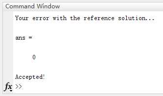
这一步的任务比较单纯,计算两个向量之间的欧式距离,将结果向量排序等。测试结果:
SIFTSimpleMatcher.m
function match = SIFTSimpleMatcher(descriptor1, descriptor2, thresh)
% SIFTSimpleMatcher
%   Match one set of SIFT descriptors (descriptor1) to another set of
%   descriptors (decriptor2). Each descriptor from descriptor1 can at
%   most be matched to one member of descriptor2, but descriptors from
%   descriptor2 can be matched more than once.
%
%   Matches are determined as follows:
%   For each descriptor vector in descriptor1, find the Euclidean distance
%   between it and each descriptor vector in descriptor2. If the smallest
%   distance is less than thresh*(the next smallest distance), we say that
%   the two vectors are a match, and we add the row [d1 index, d2 index] to
%   the "match" array.
%
% INPUT:
%   descriptor1: N1 * 128 matrix, each row is a SIFT descriptor.
%   descriptor2: N2 * 128 matrix, each row is a SIFT descriptor.
%   thresh: a given threshold of ratio. Typically 0.7
%
% OUTPUT:
%   Match: N * 2 matrix, each row is a match.
%          For example, Match(k, :) = [i, j] means i-th descriptor in
%          descriptor1 is matched to j-th descriptor in descriptor2.
    if ~exist('thresh', 'var'),
        thresh = 0.7;
    end

    match = [];
%%%%%%%%%%%%%%%%%%%%%%%%%%%%%%%%%%%%%%%%%%%%%%%%%%%%%%%%%%%%%%%%%%%%%%%%%%%%%%%%
%                                                                              %
%                                YOUR CODE HERE:                               %
%                                                                              %
%%%%%%%%%%%%%%%%%%%%%%%%%%%%%%%%%%%%%%%%%%%%%%%%%%%%%%%%%%%%%%%%%%%%%%%%%%%%%%%%
[N1,~]=size(descriptor1);
[N2,~]=size(descriptor2);
for i=1:N1
    distance=[];
    for j=1:N2
        subtract=descriptor1(i,:)-descriptor2(j,:);
        distance=[distance,norm(subtract)];
    end
        sort_distance=sort(distance);
        if(sort_distance(1)<0.7*sort_distance(2))
            j=find(distance==sort_distance(1));
            match=[match;[i,j]];
        end
end


%%%%%%%%%%%%%%%%%%%%%%%%%%%%%%%%%%%%%%%%%%%%%%%%%%%%%%%%%%%%%%%%%%%%%%%%%%%%%%%%
%                                                                              %
%                                 END YOUR CODE                                %
%                                                                              %
%%%%%%%%%%%%%%%%%%%%%%%%%%%%%%%%%%%%%%%%%%%%%%%%%%%%%%%%%%%%%%%%%%%%%%%%%%%%%%%%

end
<译>
#4.计算变换矩阵
我们现在有一个两幅图像之间匹配点的列表。我们会使用它来找到一个变换矩阵,这个矩阵能将image1的点映射到image2对应的坐标系。换句话说,如果在image1中的点 x 1 x_1 x1 y 1 y_1 y1匹配image2中的点 x 2 x_2 x2 y 2 y_2 y2,我们需要找到一个变换矩阵H
$ \begin{bmatrix} x_2 \ y_2 \ 1\end{bmatrix} =H\begin{bmatrix}x_1 \ y_1 \ 1\end{bmatrix}$
需要有足够多的点,Matlab能够帮我们计算最佳的H。复习以前的有关最小二乘法的作业。编写ComputeAffineMatrix.m,根据给定的匹配点对计算H。
运行提供的EvaluateAffineMatrix.m来检查你的实现。
采用最小二乘法求取矩阵方程的解,在Matlab上一个“反斜杠”就能够解决。
ComputeAffineMatrix.m
function H = ComputeAffineMatrix( Pt1, Pt2 )
%ComputeAffineMatrix
%   Computes the transformation matrix that transforms a point from
%   coordinate frame 1 to coordinate frame 2
%Input:
%   Pt1: N * 2 matrix, each row is a point in image 1
%       (N must be at least 3)
%   Pt2: N * 2 matrix, each row is the point in image 2 that
%       matches the same point in image 1 (N should be more than 3)
%Output:
%   H: 3 * 3 affine transformation matrix,
%       such that H*pt1(i,:) = pt2(i,:)

    N = size(Pt1,1);
    if size(Pt1, 1) ~= size(Pt2, 1),
        error('Dimensions unmatched.');
    elseif N<3
        error('At least 3 points are required.');
    end

    % Convert the input points to homogeneous coordintes.
    P1 = [Pt1';ones(1,N)];
    P2 = [Pt2';ones(1,N)];

    % Now, we must solve for the unknown H that satisfies H*P1=P2
    % But MATLAB needs a system in the form Ax=b, and A\b solves for x.
    % In other words, the unknown matrix must be on the right.
    % But we can use the properties of matrix transpose to get something
    % in that form. Just take the transpose of both sides of our equation
    % above, to yield P1'*H'=P2'. Then MATLAB can solve for H', and we can
    % transpose the result to produce H.

    H = [];
%%%%%%%%%%%%%%%%%%%%%%%%%%%%%%%%%%%%%%%%%%%%%%%%%%%%%%%%%%%%%%%%%%%%%%%%%%%%%%%%
%                                                                              %
%                                YOUR CODE HERE:                               %
%        Use MATLAB's "A\b" syntax to solve for H_transpose as discussed       %
%                     above, then convert it to the final H                    %
%                                                                              %
%%%%%%%%%%%%%%%%%%%%%%%%%%%%%%%%%%%%%%%%%%%%%%%%%%%%%%%%%%%%%%%%%%%%%%%%%%%%%%%%
    H_transpose=P1'\P2';
    H=H_transpose';
%%%%%%%%%%%%%%%%%%%%%%%%%%%%%%%%%%%%%%%%%%%%%%%%%%%%%%%%%%%%%%%%%%%%%%%
%       END OF YOUR CODE                                              %
%%%%%%%%%%%%%%%%%%%%%%%%%%%%%%%%%%%%%%%%%%%%%%%%%%%%%%%%%%%%%%%%%%%%%%%

    % Sometimes numerical issues cause least-squares to produce a bottom
    % row which is not exactly [0 0 1], which confuses some of the later
    % code. So we'll ensure the bottom row is exactly [0 0 1].
    H(3,:) = [0 0 1];
end
<译>
#5.RANSAC
我们使用RANSAC(“RANdom SAmple Consensus”)选取内点来计算单应矩阵,而不是直接把所有的SIFT关键点匹配放进ComputeAffineMatrix.m产生结果。在这里,内点是指符合相同的变换矩阵的匹配对。我们已经替你实现RANSAC,除了判断两个点适应矩阵H的符合度的函数没有给。在RANSAC.m里编写ComputeError()函数,计算 H p 1 Hp_1 Hp1和 p 2 p_2 p2之间的欧式距离。
其中, ∥ ∥ 2 \begin{Vmatrix}\end{Vmatrix}_2 ∥∥2代表欧式距离,正如上面第三部分定义的一样。在你完成RANSANCFit.m之后,你可以运行TransformationTester.m来测试你的代码。你应该得到跟图1类似的结果。
我的实现:
RANSACFit.m
function H = RANSACFit(p1, p2, match, maxIter, seedSetSize, maxInlierError, goodFitThresh )
%RANSACFit Use RANSAC to find a robust affine transformation
% Input:
%   p1: N1 * 2 matrix, each row is a point
%   p2: N2 * 2 matrix, each row is a point
%   match: M * 2 matrix, each row represents a match [index of p1, index of p2]
%   maxIter: the number of iterations RANSAC will run
%   seedNum: The number of randomly-chosen seed points that we'll use to fit
%   our initial circle
%   maxInlierError: A match not in the seed set is considered an inlier if
%                   its error is less than maxInlierError. Error is
%                   measured as sum of Euclidean distance between transformed
%                   point1 and point2. You need to implement the
%                   ComputeCost function.
%
%   goodFitThresh: The threshold for deciding whether or not a model is
%                  good; for a model to be good, at least goodFitThresh
%                  non-seed points must be declared inliers.
%
% Output:
%   H: a robust estimation of affine transformation from p1 to p2
%
%
    N = size(match, 1);
    if N<3
        error('not enough matches to produce a transformation matrix')
    end
    if ~exist('maxIter', 'var'),
        maxIter = 200;
    end
    if ~exist('seedSetSize', 'var'),
        seedSetSize = ceil(0.2 * N);
    end
    seedSetSize = max(seedSetSize,3);
    if ~exist('maxInlierError', 'var'),
        maxInlierError = 30;
    end
    if ~exist('goodFitThresh', 'var'),
        goodFitThresh = floor(0.7 * N);
    end
    H = eye(3);
    % below is an obfuscated version of RANSAC. You don't need to
    % edit any of this code, just the ComputeError() function below

    iota = Inf;
    kappa = 0;
    lambda = iota;
    alpha = seedSetSize;
    for i = 1 : maxIter,
        [beta, gamma] = part(match, alpha);
        eta = ComputeAffineMatrix(p1(beta(:, 1), :), p2(beta(:, 2), :));
        delta = ComputeError(eta, p1, p2, gamma);
        epsilon = (delta <= maxInlierError);
        if sum(epsilon(:)) + alpha >= goodFitThresh,
            zeta = [beta; gamma(epsilon, :)];
            eta = ComputeAffineMatrix(p1(zeta(:, 1), :), p2(zeta(:, 2), :));
            theta = sum(ComputeError(eta, p1, p2, zeta));
            if theta < iota,
                H = eta;
                kappa = lambda;
                iota = theta;
            end
        end
    end

    if sum(sum((H - eye(3)).^2)) == 0,
        disp('No RANSAC fit was found.')
    end
end

function dists = ComputeError(H, pt1, pt2, match)
% Compute the error using transformation matrix H to
% transform the point in pt1 to its matching point in pt2.
%
% Input:
%   H: 3 x 3 transformation matrix where H * [x; y; 1] transforms the point
%      (x, y) from the coordinate system of pt1 to the coordinate system of
%      pt2.
%   pt1: N1 x 2 matrix where each ROW is a data point [x_i, y_i]
%   pt2: N2 x 2 matrix where each ROW is a data point [x_i, y_i]
%   match: M x 2 matrix, each row represents a match [index of pt1, index of pt2]
%
% Output:
%    dists: An M x 1 vector where dists(i) is the error of fitting the i-th
%           match to the given transformation matrix.
%           Error is measured as the Euclidean distance between (transformed pt1)
%           and pt2 in homogeneous coordinates.
%%%%%%%%%%%%%%%%%%%%%%%%%%%%%%%%%%%%%%%%%%%%%%%%%%%%%%%%%%%%%%%%%%%%%%%%%%%%%%%%
%                                                                              %
%                                YOUR CODE HERE.                               %
%           Convert the points to a usable format, perform the                 %
%           transformation on pt1 points, and find their distance to their     %
%           MATCHING pt2 points.                                               %
%%%%%%%%%%%%%%%%%%%%%%%%%%%%%%%%%%%%%%%%%%%%%%%%%%%%%%%%%%%%%%%%%%%%%%%%%%%%%%%%
    % hint: If you have an array of indices, MATLAB can directly use it to
    % index into another array. For example, pt1(match(:, 1),:) returns a
    % matrix whose first row is pt1(match(1,1),:), second row is
    % pt1(match(2,1),:), etc. (You may use 'for' loops if this is too
    % confusing, but understanding it will make your code simple and fast.)
    dists = zeros(size(match,1),1);
    transform_pt1=H*[pt1(match(:,1),:)';ones(1,size(match,1))];
    subtract=pt2(match(:,2),:)-transform_pt1(1:2,:)';
    dists=sqrt(subtract(:,1).^2+subtract(:,2).^2);

%%%%%%%%%%%%%%%%%%%%%%%%%%%%%%%%%%%%%%%%%%%%%%%%%%%%%%%%%%%%%%%%%%%%%%%%%%%%%%%%
%                                                                              %
%                                 END YOUR CODE                                %
%                                                                              %
%%%%%%%%%%%%%%%%%%%%%%%%%%%%%%%%%%%%%%%%%%%%%%%%%%%%%%%%%%%%%%%%%%%%%%%%%%%%%%%%
    if size(dists,1) ~= size(match,1) || size(dists,2) ~= 1
        error('wrong format');
    end
end

function [D1, D2] = part(D, splitSize)
    idx = randperm(size(D, 1));
    D1 = D(idx(1:splitSize), :);
    D2 = D(idx(splitSize+1:end), :);
end
<译>
#6.拼接多幅图像
我们提供了一个函数,使用你之前写的代码就能高效的拼接一个有序的图像序列(多幅图像是在一条线上拍摄的,每张图像都是最终全景的一部分)。给定一个包含m张图像的序列,
I m g 1 Img_1 Img1, I m g 2 Img_2 Img2,…… I m g m Img_m Imgm,
我们的代码使用每相邻两幅图像,然后计算它们之间的变换矩阵,比如讲一个点从 I m g i Img_i Imgi的坐标系转换成 I m g i + 1 Img_{i+1} Imgi+1的坐标系。(是通过在每对图像上简单的调用你写的代码实现它的。)
我们之后选取一个参考图像 I m g r e f Img_{ref} Imgref,它处在矩阵序列的中间。我们想让我们最终的全景图处在 I m g r e f Img_{ref} Imgref的坐标系下。所以,对于对于非参考图像的 I m g i Img_{i} Imgi,我们需要一个变换矩阵,来将第i帧图像的点转换到ref帧上。(MATLAB然后能够使用这个变换矩阵,帮我们变换图像。)
你的任务是在MultipleStitch.m中,实现函数makeTransformToReferenceFrame。给你一个矩阵列表,包含i帧到i+1帧的转换关系。你必须使用这些矩阵产生一个转换给定帧到参考帧的变换矩阵。
完成了这个部分,你可以通过运行StitchTester.m来检查你的代码。你会得到跟图2相似的结果……
这个任务也相对单纯,只是用到矩阵的乘法和求逆运算。
MultipleStitch.m
function Pano = MultipleStitch( IMAGES, TRANS, fileName )
%%%%%%%%%%%%%%%%%%%%%%%%%%%%%%%%%%%%%%%%%%%%%%%%%%%%%%%%%%%%%%%%%%%%%%%%%%%%%%%
%MultipleStitch
%   This function stitches multiple images together and outputs the panoramic stitched image
%   with a chain of input images and its corresponding transformations.
%
%   Given a chain of images:
%       I1 -> I2 -> I3 -> ... -> Im
%   and its corresponding transformations:
%       T1 transforms I1 to I2
%       T2 transforms I2 to I3
%       ....
%       Tm-1 transforms Im-1 to Im
%
%   We choose the middle image as the reference image, and the outputed
%   panorama is in the same coordinate system as the reference image.
%
%   For this part, all the image stitching code has been provided to you.
%   The main task for you is to fill in the code so that current
%   transformations are used when we produce the final panorama.
%
%   Originally, we have
%       I1 -> I2 -> ... -> Iref -> ... -> Im-1 -> Im
%   When we fix Iref as the final coordinate system, we want all other
%   images transformed to Iref. You are responsible for finding the current
%   transformations used under this circumstances.
%
% INPUT:
%   IMAGES: 1 * m cell array, each cell contains an image
%   TRANS: 1 * (m-1) cell array, each cell i contains an affine
%   transformation matrix that transforms Ii to Ii+1.
%   fileName: the output file name.
%
% OUTPUT:
%   Pano: the final panoramic image.
%%%%%%%%%%%%%%%%%%%%%%%%%%%%%%%%%%%%%%%%%%%%%%%%%%%%%%%%%%%%%%%%%%%%%%%%%%%%%

if ~exist('fileName', 'var'),
    fileName = 'pano.jpg';
end

if length(IMAGES) ~= length(TRANS)+1,
    error('Number of images does not match the number of transformations.');
end

%% Outbounds of panorama image
outBounds = zeros(2,2);
outBounds(1,:) = Inf;
outBounds(2,:) = -Inf;

%% Choose reference image Iref
refIdx = ceil(median(1:length(IMAGES)));

%% Estimate the largest possible panorama size
[nrows, ncols, ~] = size(IMAGES{1});
nrows = length(IMAGES) * nrows;
ncols = length(IMAGES) * ncols;

% imageToRefTrans is a 1 x m cell array where imageToRefTrans{i} gives the
% affine transformation from IMAGES{i} to the reference image
% IMAGES{refIdx}. Your task is to fill in this array.
imageToRefTrans = cell(1, length(IMAGES));

% Initialize imageToRefTrans to contain the identity transform.
for idx = 1:length(imageToRefTrans)
    imageToRefTrans{idx} = eye(3);
end

%% Find the correct transformations used for images on the left side of Iref
for idx = refIdx-1:-1:1,
    imageToRefTrans{idx} = makeTransformToReferenceFrame(TRANS, idx, refIdx);
    T = imageToRefTrans{idx};
    tmpBounds = findbounds(maketform('affine', T'), [1 1; ncols nrows]);
    outBounds(1,:) = min(outBounds(1,:),tmpBounds(1,:));
    outBounds(2,:) = max(outBounds(2,:),tmpBounds(2,:));
end

%% Find the correct transformations used for images on the right side of Iref

for idx = refIdx + 1 : length(imageToRefTrans),
    imageToRefTrans{idx} = makeTransformToReferenceFrame(TRANS, idx, refIdx);
    T = imageToRefTrans{idx};
    T(3, :) = [0, 0, 1]; % Fix rounding errors in the last row.
    tmpBounds = findbounds(maketform('affine', T'), [1 1; ncols nrows]);
    outBounds(1,:) = min(outBounds(1,:),tmpBounds(1,:));
    outBounds(2,:) = max(outBounds(2,:),tmpBounds(2,:));
end

%% Stitch the Iref image.
XdataLimit = round(outBounds(:,1)');
YdataLimit = round(outBounds(:,2)');
Pano = imtransform( im2double(IMAGES{refIdx}), maketform('affine', eye(3)), 'bilinear', ...
                    'XData', XdataLimit, 'YData', YdataLimit, ...
                    'FillValues', NaN, 'XYScale',1);

%% Transform the images from the left side of Iref using the correct transformations you computed
for idx = refIdx-1:-1:1,
    T = imageToRefTrans{idx};
    Tform = maketform('affine', T');
    AddOn = imtransform(im2double(IMAGES{idx}), Tform, 'bilinear', ...
                        'XData', XdataLimit, 'YData', YdataLimit, ...
                        'FillValues', NaN, 'XYScale',1);
    result_mask = ~isnan(Pano(:,:,1));
    temp_mask = ~isnan(AddOn(:,:,1));
    add_mask = temp_mask & (~result_mask);

    for c = 1 : size(Pano,3),
        cur_im = Pano(:,:,c);
        temp_im = AddOn(:,:,c);
        cur_im(add_mask) = temp_im(add_mask);
        Pano(:,:,c) = cur_im;
    end
end

%% Transform the images from the right side of Iref using the correct transformations you computed
for idx = refIdx + 1 : length(imageToRefTrans),
    T = imageToRefTrans{idx};
    T(3, :) = [0, 0, 1]; % Fix rounding errors in the last row.
    Tform = maketform('affine', T');
    AddOn = imtransform(im2double(IMAGES{idx}), Tform, 'bilinear', ...
                        'XData', XdataLimit, 'YData', YdataLimit, ...
                        'FillValues', NaN, 'XYScale',1);
    result_mask = ~isnan(Pano(:,:,1));
    temp_mask = ~isnan(AddOn(:,:,1));
    add_mask = temp_mask & (~result_mask);

    for c = 1 : size(Pano,3),
        cur_im = Pano(:,:,c);
        temp_im = AddOn(:,:,c);
        cur_im(add_mask) = temp_im(add_mask);
        Pano(:,:,c) = cur_im;
    end
end

%% Cropping the final panorama to leave out black spaces.
[I, J] = ind2sub([size(Pano, 1), size(Pano, 2)], find(~isnan(Pano(:, :, 1))));
upper = max(min(I)-1, 1);
lower = min(max(I)+1, size(Pano, 1));
left = max(min(J)-1, 1);
right = min(max(J)+1, size(Pano, 2));
Pano = Pano(upper:lower, left:right,:);

imwrite(Pano, fileName);

end

function T = makeTransformToReferenceFrame(i_To_iPlusOne_Transform, currentFrameIndex, refFrameIndex)
%makeTransformToReferenceFrame
% INPUT:
%   i_To_iPlusOne_Transform: this is a cell array where
%   i_To_iPlusOne_Transform{i} contains the 3x3 homogeneous transformation
%   matrix that transforms a point in frame i to the corresponding point in
%   frame i+1
%
%   currentFrameIndex: index of the current coordinate frame in i_To_iPlusOne_Transform
%   refFrameIndex: index of the reference coordinate frame
%
% OUTPUT:
%   T: A 3x3 homogeneous transformation matrix that would convert a point
%   in the current frame into the corresponding point in the reference
%   frame. For example, if the current frame is 2 and the reference frame
%   is 3, then T = i_To_iPlusOne_Transform{2}. If the current frame and
%   reference frame are not adjacent, T will need to be calculated.


%%%%%%%%%%%%%%%%%%%%%%%%%%%%%%%%%%%%%%%%%%%%%%%%%%%%%%%%%%%%%%%%%%%%%%%%%%%%%%%%
%                                                                              %
%                 YOUR CODE HERE: Calculate T as defined above.                %
%                                                                              %
%%%%%%%%%%%%%%%%%%%%%%%%%%%%%%%%%%%%%%%%%%%%%%%%%%%%%%%%%%%%%%%%%%%%%%%%%%%%%%%%

% HINT 1: There are two separate cases to consider: currentFrameIndex <
% refFrameIndex (this is the easier case), and currentFrameIndex >
% refFrameIndex (this is the harder case).

% HINT 2: You can use the pinv function to invert a transformation.
if currentFrameIndex<refFrameIndex
    T=eye(3);
    for i=currentFrameIndex:refFrameIndex-1
        T=T*i_To_iPlusOne_Transform{i};
    end
elseif currentFrameIndex>refFrameIndex
    T=eye(3);
    for i=currentFrameIndex-1:refFrameIndex
        T=T*pinv(i_To_iPlusOne_Transform{i});
    end
else
    T=eye(3);
end


%%%%%%%%%%%%%%%%%%%%%%%%%%%%%%%%%%%%%%%%%%%%%%%%%%%%%%%%%%%%%%%%%%%%%%%%%%%%%%%%
%                                                                              %
%                               END OF YOUR CODE                               %
%                                                                              %
%%%%%%%%%%%%%%%%%%%%%%%%%%%%%%%%%%%%%%%%%%%%%%%%%%%%%%%%%%%%%%%%%%%%%%%%%%%%%%%%

end
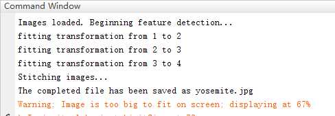
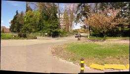
最终测试:
#拼接全景结果
今天的文章图像拼接(八):拼接多幅图像+Matlab实现+Stanford Open Course分享到此就结束了,感谢您的阅读,如果确实帮到您,您可以动动手指转发给其他人。
版权声明:本文内容由互联网用户自发贡献,该文观点仅代表作者本人。本站仅提供信息存储空间服务,不拥有所有权,不承担相关法律责任。如发现本站有涉嫌侵权/违法违规的内容, 请发送邮件至 举报,一经查实,本站将立刻删除。
如需转载请保留出处:https://bianchenghao.cn/30205.html


