
模型系列:增益模型Uplift Modeling原理和案例
目录
简介
Uplift是一种用于用户级别的治疗增量效应估计的预测建模技术。每家公司都希望增加自己的利润,而其中一个选择是激励客户购买//消费或识别理想的客户。
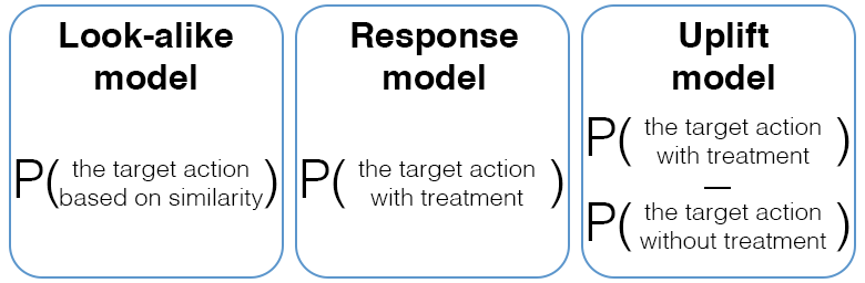
1. 类似模型 Look-alike model
基本情况是使用类似建模。我们可以通过与具有相同特征的先前客户进行比较来了解客户的行为,例如年龄、教育(我们对他们了解的内容以及他们愿意透露的内容)。这种方法需要我们的消费者数据和完成的操作以及一些随机数据,例如在我们的商店中没有购买任何东西但在其他商店中购买了东西的客户的数据。使用这种方法和机器学习,我们试图在新数据中找到与我们类似的客户,他们将成为我们促销的主要目标。
2. 响应模型 Response model
响应建模评估可能在治疗后完成行动的客户。因此,我们收集了治疗(沟通)后的数据,并知道积极和消极的观察结果。有些人购买了我们的产品,其他人没有。使用这些数据和机器学习,我们试图获得客户在治疗后完成所需行动的概率。
3. Uplift建模 Uplift model
最后但并非最不重要的是增益模型。与响应模型相比,增益模型评估沟通(治疗)的净效应,并尝试仅选择在治疗后才完成行动的客户。这组模型估计了具有沟通(治疗)和没有治疗的客户之间行为差异。我们将详细介绍这些模型。
首先,我们将行动表示为 Y(1 - 行动,0 - 无行动),治疗表示为 W(1 - 治疗,0 - 无治疗)

我们可以将客户分为4个具有相同行为的群体:
🤷 将采取行动 - 这群人无论如何都会采取行动(Y=1, W=1和Y=1, W=0)
🙋 可说服的 - 这群人只有在治疗后才会采取行动(Y=1, W=1和Y=0, W=0)
🙅 不要打扰 - 这群人会在没有治疗的情况下执行某个行动,但在治疗后可能会结束(Y=1, W=0和Y=0, W=1)
🤦 永远不会回应 - 这群人不在乎治疗(Y=0, W=1和Y=0, W=0)
对于客户来说,因果效应是其在有治疗和无治疗情况下结果的差异:
$ \tau_i = Y^1_i - Y^0_i $
对于更有趣的目的,对于客户群体来说,因果效应是有治疗和无治疗情况下该群体预期结果的差异 - CATE(条件平均处理效应):
$ CATE = E[Y^1_i|X_i] - E[Y^0_i|X_i] $
然而,我们不能同时观察这两种情况,只能在不同的宇宙中。这就是为什么我们只能估计 C A T E ^ \widehat{CATE} CATE
像往常一样:
$ \widehat{CATE} (uplift) = E[Y_i|X_i = x, W_i = 1] - E[Y_i|X_i = x, W_i = 0] $,其中 $ Y^1_i = Y_i = Y^1_i if W_i = 1$ and Y i 0 Y^0_i Yi0 where $W_i = 0 $
注意! W i W_i Wi 应该在给定 X i X_i Xi 的条件下与 Y i 1 Y^1_i Yi1 和 Y i 0 Y^0_i Yi0 独立。
有两种类型的增益模型:
学习器- 转换问题并使用经典的机器学习模型直接增益模型- 直接预测增益的算法。
1. 初步步骤
import numpy as np import pandas as pd from matplotlib import pyplot as plt from tqdm.notebook import tqdm import seaborn as sns from statsmodels.graphics.gofplots import plot !pip install scikit-uplift -q from sklift.metrics import uplift_at_k, uplift_auc_score, qini_auc_score, weighted_average_uplift from sklift.viz import plot_uplift_preds from sklift.models import SoloModel, TwoModels import xgboost as xgb [33mWARNING: Running pip as the 'root' user can result in broken permissions and conflicting behaviour with the system package manager. It is recommended to use a virtual environment instead: https://pip.pypa.io/warnings/venv[0m # 读取csv文件,并将其存储在train变量中 train = pd.read_csv('../input/megafon-uplift-competition/train (1).csv') 我们看到了许多隐藏的特征X_1-X_50,二处理(以对象格式)和二转换
# 查看训练数据的前几行 train.head() | id | treatment_group | X_1 | X_2 | X_3 | X_4 | X_5 | X_6 | X_7 | X_8 | ... | X_42 | X_43 | X_44 | X_45 | X_46 | X_47 | X_48 | X_49 | X_50 | conversion | |
|---|---|---|---|---|---|---|---|---|---|---|---|---|---|---|---|---|---|---|---|---|---|
| 0 | 0 | control | 39. | -0. | 19. | 21. | 55. | 182. | -5. | 144. | ... | 134. | -213. | -2.092461 | -93. | -0. | -312. | 44. | -125. | 16. | 0 |
| 1 | 1 | control | 38. | 0. | -42.064512 | -48. | -33. | 179. | -87. | -162. | ... | 72. | 559. | 1. | 80.037124 | -1. | -111. | -127. | -117. | 10. | 0 |
| 2 | 2 | treatment | -16. | 1. | -8. | -18. | -22. | -116. | -63. | -38. | ... | 2. | 96. | 1. | -33. | 0. | -679. | -91.009397 | -18. | 14. | 0 |
| 3 | 3 | treatment | -72.040154 | -0. | 39. | 16. | -1. | 68. | 23.073147 | 4. | ... | 83. | -323. | -0. | 93. | -1. | -442. | -22. | -75. | 11. | 0 |
| 4 | 4 | treatment | 18. | 0. | 24. | -34. | 24. | -155. | -12. | 26. | ... | -208. | 118. | -0. | -117. | 1. | 627. | 122.019189 | 194.091195 | -11. | 0 |
5 rows × 53 columns
# 对训练数据集进行信息描述 train.info() <class 'pandas.core.frame.DataFrame'> RangeIndex: entries, 0 to Data columns (total 53 columns): # Column Non-Null Count Dtype --- ------ -------------- ----- 0 id non-null int64 1 treatment_group non-null object 2 X_1 non-null float64 3 X_2 non-null float64 4 X_3 non-null float64 5 X_4 non-null float64 6 X_5 non-null float64 7 X_6 non-null float64 8 X_7 non-null float64 9 X_8 non-null float64 10 X_9 non-null float64 11 X_10 non-null float64 12 X_11 non-null float64 13 X_12 non-null float64 14 X_13 non-null float64 15 X_14 non-null float64 16 X_15 non-null float64 17 X_16 non-null float64 18 X_17 non-null float64 19 X_18 non-null float64 20 X_19 non-null float64 21 X_20 non-null float64 22 X_21 non-null float64 23 X_22 non-null float64 24 X_23 non-null float64 25 X_24 non-null float64 26 X_25 non-null float64 27 X_26 non-null float64 28 X_27 non-null float64 29 X_28 non-null float64 30 X_29 non-null float64 31 X_30 non-null float64 32 X_31 non-null float64 33 X_32 non-null float64 34 X_33 non-null float64 35 X_34 non-null float64 36 X_35 non-null float64 37 X_36 non-null float64 38 X_37 non-null float64 39 X_38 non-null float64 40 X_39 non-null float64 41 X_40 non-null float64 42 X_41 non-null float64 43 X_42 non-null float64 44 X_43 non-null float64 45 X_44 non-null float64 46 X_45 non-null float64 47 X_46 non-null float64 48 X_47 non-null float64 49 X_48 non-null float64 50 X_49 non-null float64 51 X_50 non-null float64 52 conversion non-null int64 dtypes: float64(50), int64(2), object(1) memory usage: 242.6+ MB 特征没有标准化或归一化
# 使用describe()函数对训练数据集进行描述性统计分析 train.describe() | id | X_1 | X_2 | X_3 | X_4 | X_5 | X_6 | X_7 | X_8 | X_9 | ... | X_42 | X_43 | X_44 | X_45 | X_46 | X_47 | X_48 | X_49 | X_50 | conversion | |
|---|---|---|---|---|---|---|---|---|---|---|---|---|---|---|---|---|---|---|---|---|---|
| count | .000000 | .000000 | .000000 | .000000 | .000000 | .000000 | .000000 | .000000 | .000000 | .000000 | ... | .000000 | .000000 | .000000 | .000000 | .000000 | .000000 | .000000 | .000000 | .000000 | .000000 |
| mean | . | -3. | 0.000405 | 0. | -1.004378 | 3. | -6. | -2. | -6. | -0.061507 | ... | -6. | 8. | 0.001296 | 0.007967 | -0.000966 | -22. | -5. | 6. | -1. | 0. |
| std | . | 54. | 0. | 31. | 45. | 53. | 140. | 59. | 74. | 44. | ... | 137.025868 | 262. | 1.000368 | 71. | 0. | 500. | 130. | 141. | 21. | 0. |
| min | 0.000000 | -271. | -4. | -148. | -244. | -302. | -683. | -322. | -506. | -218. | ... | -633. | -1345. | -4. | -360. | -4. | -2506. | -687. | -702. | -98.094323 | 0.000000 |
| 25% | . | -40. | -0. | -20. | -30. | -31. | -100. | -42. | -54. | -30. | ... | -99.033996 | -167. | -0. | -48. | -0. | -357. | -93. | -88. | -15. | 0.000000 |
| 50% | . | -3. | 0.000915 | 0. | -0. | 3. | -6. | -2. | -6. | -0. | ... | -6. | 8. | 0.001639 | 0.045537 | -0.002251 | -20. | -5. | 6. | -1. | 0.000000 |
| 75% | . | 33. | 0. | 21. | 29.027860 | 38. | 88. | 37. | 41. | 30. | ... | 85. | 185. | 0. | 48. | 0. | 313. | 81. | 101. | 13. | 0.000000 |
| max | .000000 | 250. | 5.062006 | 170.053291 | 235.095937 | 284. | 656. | 293. | 550. | 219. | ... | 689. | 1488. | 4. | 384. | 5.086304 | 2534. | 595. | 630. | 112. | 1.000000 |
8 rows × 52 columns
然而,很有可能这些特征已经被清除。每个特征分布看起来都很正常。
# 给代码添加中文注释 # 设置行数和列数 rows, cols = 10, 5 # 创建一个包含多个子图的图形对象,并设置图形的大小 f, axs = plt.subplots(nrows=rows, ncols=cols, figsize=(20, 25)) # 设置图形的背景颜色为白色 f.set_facecolor("#fff") # 设置特征数量为1 n_feat = 1 # 遍历每一行 for row in tqdm(range(rows)): # 遍历每一列 for col in range(cols): try: # 绘制核密度估计图,并设置填充、透明度、线宽、边缘颜色等参数 sns.kdeplot(x=f'X_{
     n_feat}', fill=True, alpha=1, linewidth=3, edgecolor="#", data=train, ax=axs[row, col], color='w') # 设置子图的背景颜色为深绿色,并设置透明度 axs[row, col].patch.set_facecolor("#619b8a") axs[row, col].patch.set_alpha(0.8) # 设置子图的网格颜色和透明度 axs[row, col].grid(color="#", alpha=1, axis="both") except IndexError: # 隐藏最后一个空图 axs[row, col].set_visible(False) # 特征数量加1 n_feat += 1 # 显示图形 f.show()
0%| | 0/10 [00:00<?, ?it/s] 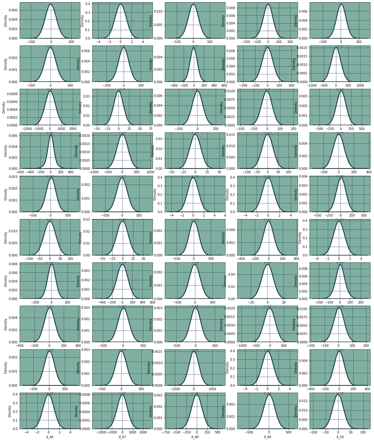
只是为了确保,请看图。
# 设置子图的行数和列数 rows, cols = 10, 5 # 创建一个包含子图的图像对象 f, axs = plt.subplots(nrows=rows, ncols=cols, figsize=(20, 25)) # 设置图像的背景颜色为白色 f.set_facecolor("#fff") # 设置特征数量为1 n_feat = 1 # 遍历每一行 for row in tqdm(range(rows)): # 遍历每一列 for col in range(cols): try: # 绘制核密度估计图 # sns.kdeplot(x=f'X_{n_feat}', fill=True, alpha=1, linewidth=3,  # edgecolor="#", data=train, ax=axs[row, col], color='w') # 绘制图 plot(train[f'X_{
     n_feat}'], ax=axs[row, col], line='q') # 设置网格线的颜色为深绿色 axs[row, col].grid(color="#", alpha=1, axis="both") # 如果索引超出范围,则隐藏最后一个空图 except IndexError: axs[row, col].set_visible(False) # 特征数量加1 n_feat += 1 # 显示图像 f.show()
0%| | 0/10 [00:00<?, ?it/s] 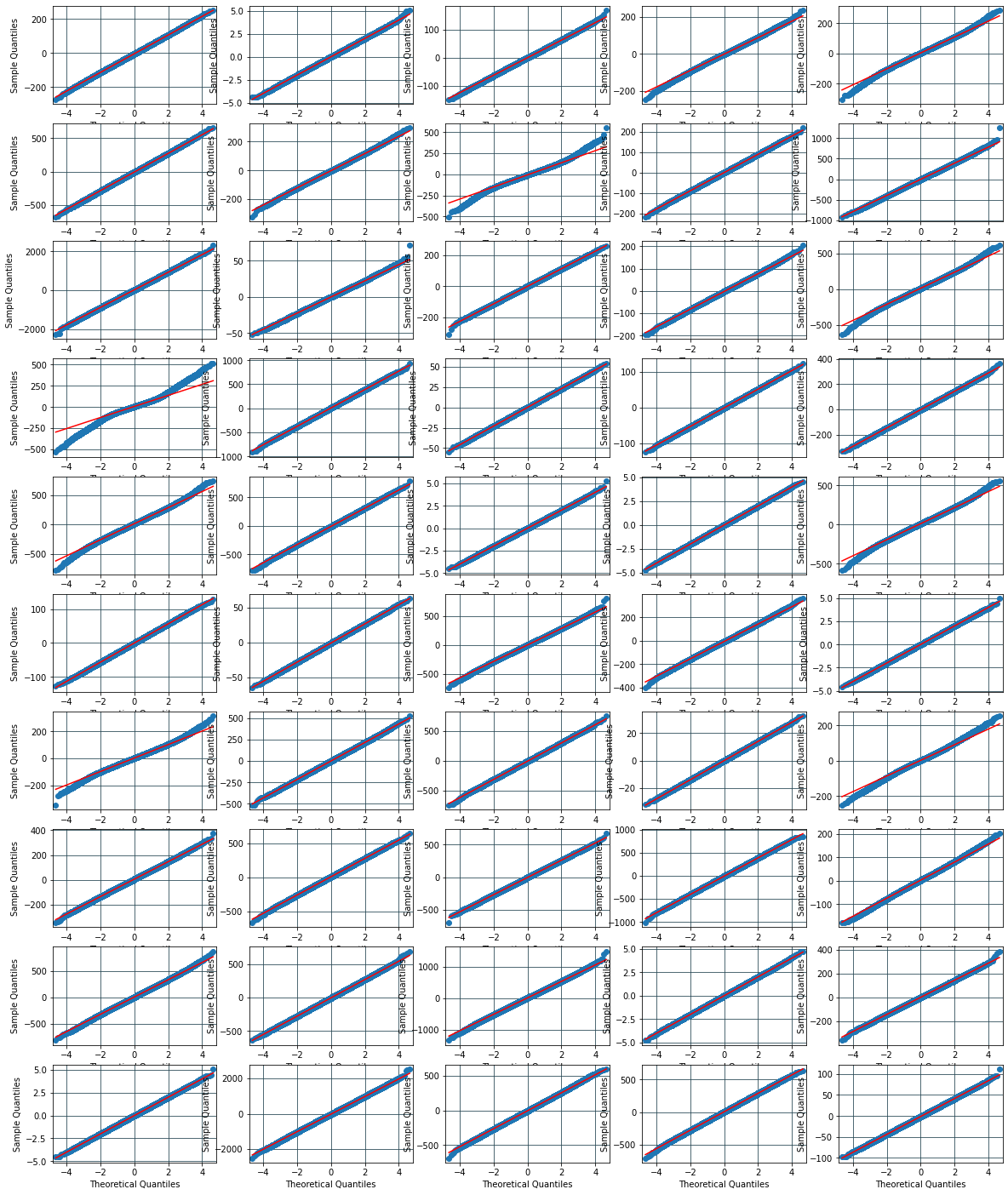
接下来让我们集中精力进行建模。
2. 指标
由于我们在研究之前没有Uplift,我们不能使用经典的Meta-Learners指标。然而,我们需要比较模型并了解它们的准确性。
1. Uplift@k
我们所需要做的就是对值进行排序(降序),并计算治疗组和对照组中目标变量(Y)的平均差异:
U p l i f t @ k = m e a n ( Y t r e a t m e n t @ k ) − m e a n ( Y c o n t r o l @ k ) Uplift@k = mean(Y^{treatment}@k) - mean(Y^{control}@k) Uplift@k=mean(Ytreatment@k)−mean(Ycontrol@k)
Y @ k Y@k Y@k - 前k%的目标变量
2. 按百分位数(十分位数)计算Uplift
相同的方法,但这里我们分别计算每个十分位数的差异
使用按百分位数计算的Uplift,我们可以计算加权平均Uplift:
加权平均Uplift$ = \frac{N^T_i * uplift_i}{\sum{N^T_i}} $
N i T N^T_i NiT - i百分位数中治疗组的大小
3. Uplift曲线和AUUC
Uplift曲线是一个依赖于对象数量的累积Uplift函数:
uplift curve i = ( Y t T N t T − Y t C N t C ) ( N t T + N t C ) \text{uplift curve}_i = (\frac{Y^T_t}{N^T_t}-\frac{Y^C_t}{N^C_t}) (N^T_t + N^C_t) uplift curvei=(NtTYtT−NtCYtC)(NtT+NtC)
其中 t − 累积对象数量 , N − T和C组的大小 \text{其中 } t - \text{累积对象数量}, N - \text{T和C组的大小} 其中 t−累积对象数量,N−T和C组的大小
AUUC - Unplift曲线下的面积是随机Uplift曲线和模型曲线之间的面积,通过理想Uplift曲线下的面积进行归一化
4. Qini曲线和AUQC
Qini曲线是另一种累积函数的方法:
qini curve i = Y t T − Y t C N t T N t C \text{qini curve}_i = Y^T_t-\frac{Y^C_tN^T_t}{N^C_t} qini curvei=YtT−NtCYtCNtT
AUQC或Qini系数 - Qini曲线下的面积是随机Qini曲线和模型曲线之间的面积,通过理想Qini曲线下的面积进行归一化
train.columns Index(['id', 'treatment_group', 'X_1', 'X_2', 'X_3', 'X_4', 'X_5', 'X_6', 'X_7', 'X_8', 'X_9', 'X_10', 'X_11', 'X_12', 'X_13', 'X_14', 'X_15', 'X_16', 'X_17', 'X_18', 'X_19', 'X_20', 'X_21', 'X_22', 'X_23', 'X_24', 'X_25', 'X_26', 'X_27', 'X_28', 'X_29', 'X_30', 'X_31', 'X_32', 'X_33', 'X_34', 'X_35', 'X_36', 'X_37', 'X_38', 'X_39', 'X_40', 'X_41', 'X_42', 'X_43', 'X_44', 'X_45', 'X_46', 'X_47', 'X_48', 'X_49', 'X_50', 'conversion'], dtype='object') # 获取'treatment_group'列的唯一值 train['treatment_group'].unique() array(['control', 'treatment'], dtype=object) # 将'treatment_group'列中的值转换为0或1,如果值为'treatment'则转换为1,否则转换为0 train['treatment_group'] = train['treatment_group'].apply(lambda x: 1 if x=='treatment' else 0) # 从sklearn库中导入train_test_split函数 from sklearn.model_selection import train_test_split # 将train数据集的前行赋值给train变量 train = train[:] # 从train数据集中选取名为'X_i'的特征列,其中i的取值范围为1到50,并将结果赋值给X变量 X = train[[f'X_{
i}' for i in range(1, 51)]] # 从train数据集中选取名为'treatment_group'的特征列,并将结果赋值给treatment变量 treatment = train['treatment_group'] # 从train数据集中选取名为'conversion'的特征列,并将结果赋值给y变量 y = train['conversion'] # 使用train_test_split函数将X、y和treatment按照指定的比例划分为训练集和验证集,并将划分结果分别赋值给X_train、X_val、y_train、y_val、treatment_train和treatment_val变量 X_train, X_val, y_train, y_val, treatment_train, treatment_val = train_test_split(X, y, treatment, test_size=0.2) 3. 学习者
3.1 S-Learner
3.1 S-学习者
S-learner的主要思想是使用特征、二进制处理(W)和二进制目标动作(Y)训练一个模型。然后使用常数W=1和W=0对测试数据进行预测。差异即为提升效果。
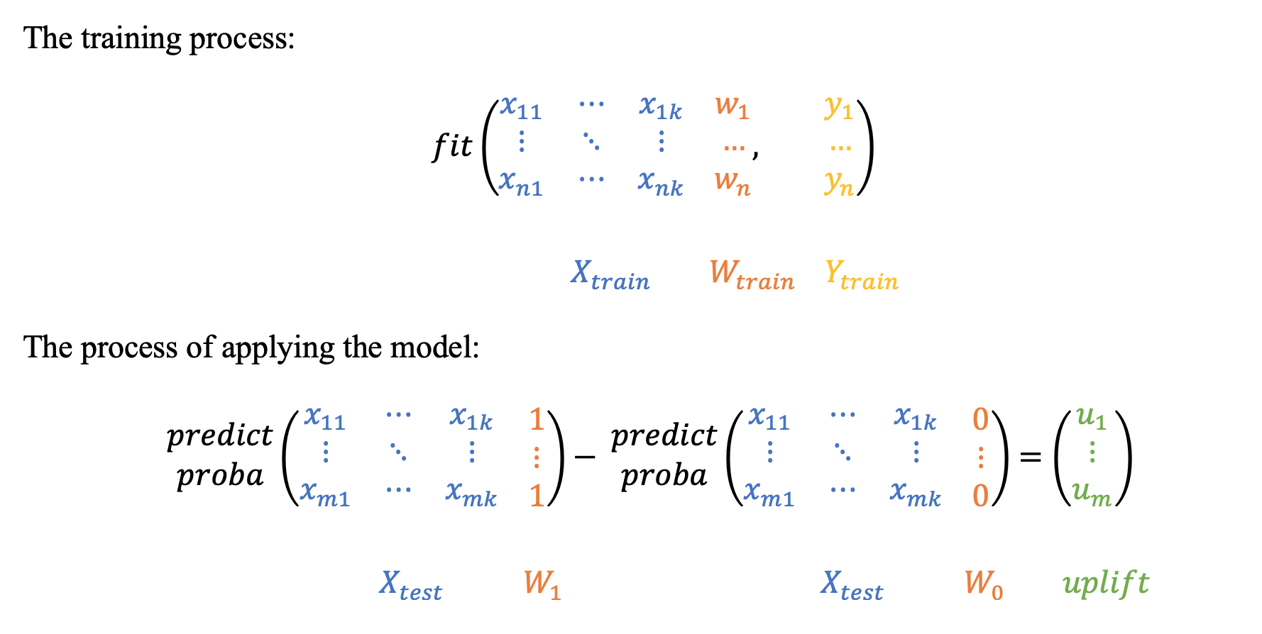
好消息是我们可以使用经典的机器学习分类器!让我们使用xgboost来做吧。你也可以尝试其他分类器并比较结果。
# 定义一个函数get_metrics,接受三个参数y_val, uplift, treatment_val def get_metrics(y_val, uplift, treatment_val): # 计算指标 # 计算前30%的提升值。按照组别排序控制组和处理组。整体排序。 upliftk = uplift_at_k(y_true=y_val, uplift=uplift, treatment=treatment_val, strategy='by_group', k=0.3) upliftk_all = uplift_at_k(y_true=y_val, uplift=uplift, treatment=treatment_val, strategy='overall', k=0.3) # 计算Qini系数 qini_coef = qini_auc_score(y_true=y_val, uplift=uplift, treatment=treatment_val) # 默认策略 - 整体排序 # 计算提升曲线下面积 uplift_auc = uplift_auc_score(y_true=y_val, uplift=uplift, treatment=treatment_val) # 计算加权平均提升值 wau = weighted_average_uplift(y_true=y_val, uplift=uplift, treatment=treatment_val, strategy='by_group') wau_all = weighted_average_uplift(y_true=y_val, uplift=uplift, treatment=treatment_val) # 打印结果 print(f'uplift at top 30% by group: {
     upliftk:.2f} by overall: {
     upliftk_all:.2f}\n', f'Weighted average uplift by group: {
     wau:.2f} by overall: {
     wau_all:.2f}\n', f'AUUC by group: {
     uplift_auc:.2f}\n', f'AUQC by group: {
     qini_coef:.2f}\n') # 返回一个包含指标结果的字典 return {
   'uplift@30': upliftk, 'uplift@30_all': upliftk_all, 'AUQC': qini_coef, 'AUUC': uplift_auc, 'WAU': wau, 'WAU_all': wau_all}
# 创建一个XGBoost分类器模型,设置随机种子为42,目标函数为二逻辑回归,禁用标签编码 xgb_sm = xgb.XGBClassifier(random_state=42, objective='binary:logistic', use_label_encoder=False) # 创建一个SoloModel对象,使用上面创建的XGBoost分类器模型作为估计器 sm = SoloModel(estimator=xgb_sm) # 使用训练数据集X_train、y_train和treatment_train来拟合SoloModel模型 sm = sm.fit(X_train, y_train, treatment_train, estimator_fit_params={
}) # 使用拟合好的SoloModel模型对验证数据集X_val进行预测 uplift_sm = sm.predict(X_val) # 使用get_metrics函数计算验证数据集的评估指标,包括y_val、uplift_sm和treatment_val res = get_metrics(y_val, uplift_sm, treatment_val) [12:14:57] WARNING: ../src/learner.cc:1115: Starting in XGBoost 1.3.0, the default evaluation metric used with the objective 'binary:logistic' was changed from 'error' to 'logloss'. Explicitly set eval_metric if you'd like to restore the old behavior. uplift at top 30% by group: 0.18 by overall: 0.18 Weighted average uplift by group: 0.04 by overall: 0.04 AUUC by group: 0.15 AUQC by group: 0.21 3.2 T-Learner
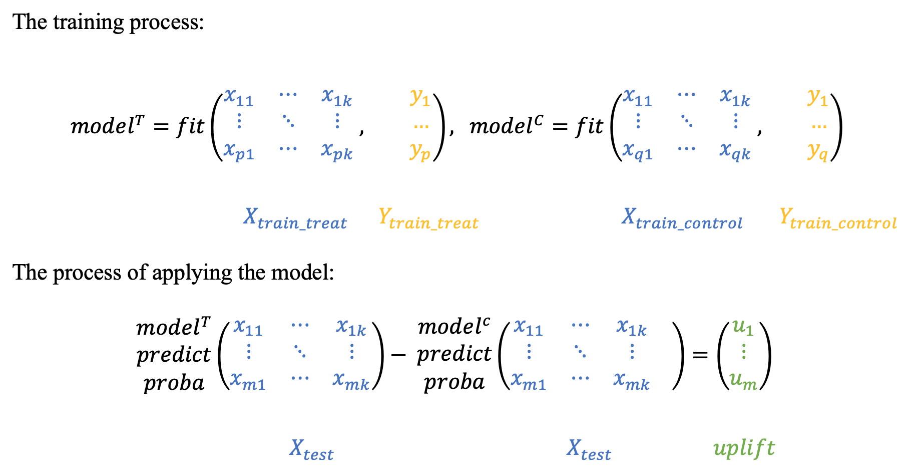
3.2 T学习器
T-learner的主要思想是训练两个独立的模型:一个基于治疗后的观察数据(T),另一个基于对照组数据(C)。提升效果是模型T和模型C在数据上的预测差异。
 # 初始化两个xgboost分类器,分别用于处理treatment组和control组 xgb_T = xgb.XGBClassifier(random_state=42, objective='binary:logistic', use_label_encoder=False) xgb_C = xgb.XGBClassifier(random_state=42, objective='binary:logistic', use_label_encoder=False) # 初始化TwoModels类,将treatment组和control组的分类器传入 sm = TwoModels(estimator_trmnt=xgb_T, estimator_ctrl=xgb_C) # 使用训练数据拟合模型 sm = sm.fit(X_train, y_train, treatment_train, estimator_trmnt_fit_params={
   }, estimator_ctrl_fit_params={
   }) # 对验证集进行预测 uplift_sm = sm.predict(X_val) # 计算模型的评估指标 res = get_metrics(y_val, uplift_sm, treatment_val)
[12:15:47] WARNING: ../src/learner.cc:1115: Starting in XGBoost 1.3.0, the default evaluation metric used with the objective 'binary:logistic' was changed from 'error' to 'logloss'. Explicitly set eval_metric if you'd like to restore the old behavior. [12:16:11] WARNING: ../src/learner.cc:1115: Starting in XGBoost 1.3.0, the default evaluation metric used with the objective 'binary:logistic' was changed from 'error' to 'logloss'. Explicitly set eval_metric if you'd like to restore the old behavior. uplift at top 30% by group: 0.17 by overall: 0.17 Weighted average uplift by group: 0.04 by overall: 0.04 AUUC by group: 0.13 AUQC by group: 0.18 结果比S-learner稍差。
3.3 T-Learner依赖模型
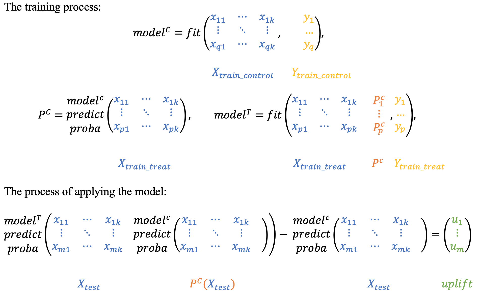
这种方法有两种可能的实现方式:基于C模型中的T-probs和基于T模型中的C-probs:
- u p l i f t i = P T ( x i , P C ( X ) ) − P C ( x i ) uplift_i = P^T(x_i, P^C(X)) - P^C(x_i) uplifti=PT(xi,PC(X))−PC(xi)
- u p l i f t i = P T ( x i ) − P C ( x i , P T ( x i ) ) uplift_i = P^T(x_i) - P^C(x_i, P^T(x_i)) uplifti=PT(xi)−PC(xi,PT(xi))
第一种方法:
 # 创建两个XGBClassifier对象,分别作为treatment模型和control模型 xgb_T = xgb.XGBClassifier(random_state=42, objective='binary:logistic', use_label_encoder=False) xgb_C = xgb.XGBClassifier(random_state=42, objective='binary:logistic', use_label_encoder=False) # 创建TwoModels对象,将treatment模型和control模型传入,并指定方法为'ddr_control' sm = TwoModels(estimator_trmnt=xgb_T, estimator_ctrl=xgb_C, method='ddr_control') # 使用训练数据拟合TwoModels对象 sm = sm.fit(X_train, y_train, treatment_train, estimator_trmnt_fit_params={
   }, estimator_ctrl_fit_params={
   }) # 使用拟合好的TwoModels对象对验证数据进行预测 uplift_sm = sm.predict(X_val) # 使用预测结果和验证数据计算评估指标 res = get_metrics(y_val, uplift_sm, treatment_val)
[12:16:37] WARNING: ../src/learner.cc:1115: Starting in XGBoost 1.3.0, the default evaluation metric used with the objective 'binary:logistic' was changed from 'error' to 'logloss'. Explicitly set eval_metric if you'd like to restore the old behavior. [12:17:02] WARNING: ../src/learner.cc:1115: Starting in XGBoost 1.3.0, the default evaluation metric used with the objective 'binary:logistic' was changed from 'error' to 'logloss'. Explicitly set eval_metric if you'd like to restore the old behavior. uplift at top 30% by group: 0.17 by overall: 0.17 Weighted average uplift by group: 0.04 by overall: 0.04 AUUC by group: 0.12 AUQC by group: 0.18 第二种方法:
 # 创建两个XGBoost分类器,用于处理treatment组和control组 xgb_T = xgb.XGBClassifier(random_state=42, objective='binary:logistic', use_label_encoder=False) xgb_C = xgb.XGBClassifier(random_state=42, objective='binary:logistic', use_label_encoder=False) # 创建TwoModels对象,使用xgb_T和xgb_C作为估计器,并选择ddr_treatment方法 sm = TwoModels(estimator_trmnt=xgb_T, estimator_ctrl=xgb_C, method='ddr_treatment') # 使用训练数据拟合TwoModels对象 sm = sm.fit(X_train, y_train, treatment_train, estimator_trmnt_fit_params={
   }, estimator_ctrl_fit_params={
   }) # 对验证数据进行预测 uplift_sm = sm.predict(X_val) # 计算模型的评估指标 res = get_metrics(y_val, uplift_sm, treatment_val)
[12:17:27] WARNING: ../src/learner.cc:1115: Starting in XGBoost 1.3.0, the default evaluation metric used with the objective 'binary:logistic' was changed from 'error' to 'logloss'. Explicitly set eval_metric if you'd like to restore the old behavior. [12:17:51] WARNING: ../src/learner.cc:1115: Starting in XGBoost 1.3.0, the default evaluation metric used with the objective 'binary:logistic' was changed from 'error' to 'logloss'. Explicitly set eval_metric if you'd like to restore the old behavior. uplift at top 30% by group: 0.17 by overall: 0.17 Weighted average uplift by group: 0.04 by overall: 0.04 AUUC by group: 0.13 AUQC by group: 0.19
版权声明:本文内容由互联网用户自发贡献,该文观点仅代表作者本人。本站仅提供信息存储空间服务,不拥有所有权,不承担相关法律责任。如发现本站有涉嫌侵权/违法违规的内容, 请发送邮件至 举报,一经查实,本站将立刻删除。
如需转载请保留出处:https://bianchenghao.cn/bian-cheng-ji-chu/85269.html