• 目前的算法包虽然可以直接使用，但速度慢，定制性差

由于Uplift模型还未被广泛使用，业界对于该技术的定义混乱，每个领域甚至每个公司都会有自己的魔改版本，甚至连该方法的名称都没有得到统一，举几个常见的例子：

• Estimating heterogeneous treatment effects (Example)
• Incremental response modeling (Example)
• Net scoring (Example)
• True response modeling (Example)

推荐使用的Packages：

• CasualML: Uplift Modeling Python Package by Uber
• Pylift Uplift Meta-learner Python Package
• R Uplift Package
• Opossum: a Python package to create synthetic uplift datasets
• “EconML” (ALICE: Automated Learning and Intelligence for Causation and Economics)
• DoWhy
• pymatch

---

---

1 pylift 模型介绍

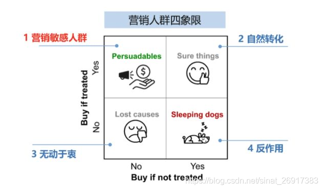
Uplift models需要每一个人的两方面信息：是否给予treatment，产出label。理想情况下，我们可以得到一些个体在随机分配到实验组（treat group）和对照组（control group）后的数据，基于他们对于treatment的反应，outcome label可以被转化为下面这个矩阵(Athey and Imbens 2016)（实际情况中可以有其他的正负样本划分方法）：

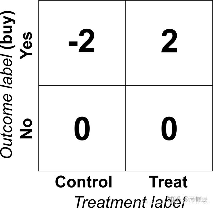
可能在第一眼的时候觉得这个目标矩阵不太靠谱，像拍脑袋的结果，为啥没有买的给不给treatment都是0？
为什么给了treatment买了就是2？
看起来非常不直观，但是是有道理在里面的，假如将一群人随机分为控制组和对照组，最后得到的平均值矩阵就是这群人的lift。

为了说明这个问题，考虑有一群人，人数为2n，其中n个给了treatment t，另外n个不给作为对照组。为了简单起见我们将i =1 ,…, n为treatment组，i =n+1 ,…, 2n为控制对照组。对于每一个用户，原始的outcomes和转换后的分别为 Yi和Zi ，那么对于这群人，对于购买行为的lift为:

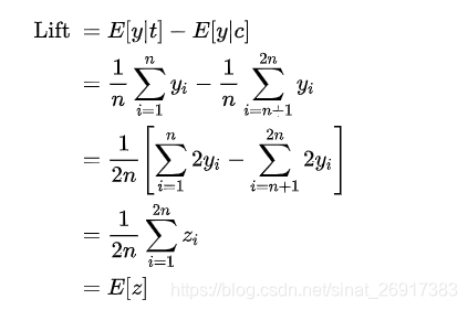
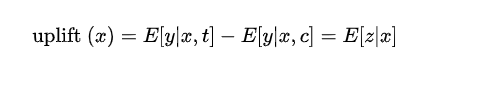
也就是说，转化后的outcome取决于前一个group的lift，这个优雅的转换大大简化了lift问题，我们可以直接对z建立回归模型，我们就可以得到对于基于特征x表征的用户的uplift：

---

2 pylift安装与Quick start

2.1 pylift的安装

Pylift是uplift建模的Python工具包。Pylift在sklearn的基础上针对uplift modeling对各模型做了一些优化，同时集成了一套uplift评价指标体系。所以Pylift内核还是sklearn，在sklearn外面封装了一套API，针对树模型做了uplift优化，可以通过Pylift实现直接的uplift modeling.

最便捷的安装方式：

pip install pylift 

2.2 pylift的Quick start

参考：【营销增益模型实战-Uplift Model原理及应用】

from pylift import TransformedOutcome up = TransformedOutcome(df1, col_treatment='Treatment', col_outcome='Converted') up.randomized_search() # 对所有参数grid search，十分耗时，使用时注意限制参数searching的数量 up.fit(up.rand_search_.best_params_) up.plot(plot_type='aqini', show_theoretical_max=True) # 绘制aqini曲线 print(up.test_results_.Q_aqini) 

up = TransformedOutcome(df, col_treatment='Treatment', col_outcome='Converted', sklearn_model=RandomForestRegressor) 

参数col_treatment是指数据集df中区分是否是treatment group的字段，通过0/1二值区分，
col_outcome相当于label字段，如有转化是1，无转化是0.
Pylift另一个方便之处是提供了计算uplift评价指标的函数。如果是使用TransformedOutcome生成的结果，直接输入up.plot(plot_type='qini')即可绘制qini曲线。如果是自己的数据，可以通过下述方式来绘制曲线：

from pylift.eval import UpliftEval upev = UpliftEval(treatment, outcome, predictions) upev.plot(plot_type='aqini') 

其中treatment标识是否treatment group，list格式；
outcome相当于label，list格式；
predictions是预测的uplift score分数，
注意这是uplift score，如果不是uplift score需要自己先将uplift score计算好。
上一小节模型评估中的图均是通过UpliftEval绘制的。

plot_type参数是绘制曲线的类型，可以绘制以下六种曲线：

• qini：qini曲线
• aqini：修正后的qini曲线，更适应treatment group和control group数据不均衡的数据
• cuplift：累积uplift曲线
• uplift：uplift曲线，不累积
• cgains：累积gain曲线
• balance：每个百分比下，实验组目标人数除以所有人数

通过以下方式计算曲线面积：

upev.Q_aqini # aqini曲线与random line之间的面积 upev.q1_qini # qini曲线与理想曲线之间的面积 upev.q2_cgains # cgains曲线与最佳实践曲线之间的面积 

Pylift用于实验很方便，但因为还是基于sklearn，当达到千万量级的数据量时，还是需要考虑分布式。

---

3 案例一：完整demo案例

来自官方github之中:simulated_data/sample.ipynb

3.1 生成模拟数据

import numpy as np, matplotlib as mpl, matplotlib.pyplot as plt, pandas as pd from pylift import TransformedOutcome from pylift.generate_data import dgp # Generate some data. df = dgp(N=10000, discrete_outcome=True) df 

数据样式：

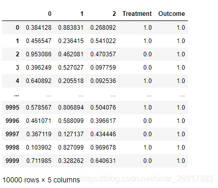
treatment是指数据集df中区分是否是treatment group的字段，通过0/1二值区分，
outcome相当于label字段，如有转化是1，无转化是0.

3.2 初始化模型

# Specify your dataframe, treatment column, and outcome column. up = TransformedOutcome(df, col_treatment='Treatment', col_outcome='Outcome', stratify=df['Treatment']) 

为了建立建模的框架，只需实例化TransformedOutcome对象，并指定实验组（treatment）和对照组（outcome）(必须输入:pandas.DataFrame)。

还有一些可选参数，可以自由调节。

其中,stratify参数比较重要，因为其会直接传递给sklearn.model_select .train_test_split用来作为训练集/验证集的拆分

3.3 数据EDA 与 特征选择

增益模型的EDA是比较有技巧性的，该库作者已经融合了一些方法进来进行特征选择和检查模型数据。

其中,NIV(net information value) 和 NWOE(net weight of evidence) 两个指标会被计算，两个指标的概念可参考这篇博客：Data Exploration with Weight of Evidence and Information Value in R

来看看这篇博客描述这两个指标：

• NIV measures the strength of a given variable
• while NWOE describes the pattern of the relationship.

Specifically, the higher the value of NIV, the better the given variable is at separating self-selectors – i.e., people who are self-motivated to buy – and persuadables that need to be motivated.

具体来说，NIV的值越高，给到的特征越能辨别出自然转化（self-selectors）与营销敏感人群（persuadables）

# This function randomly shuffles your training data set and calculates net information value. up.NIV()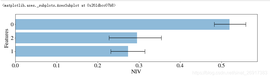 

up.NWOE(feats_to_use=[0])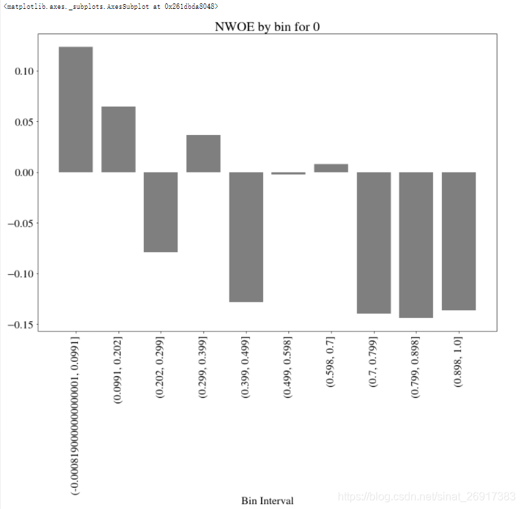 

3.4 超参数优化与模型拟合

up.randomized_search(n_iter=20, n_jobs=10, random_state=1) up.fit(up.rand_search_.best_params_)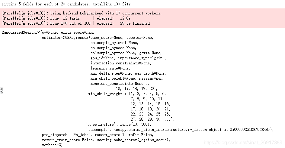 

3.5 模型评估

up.plot()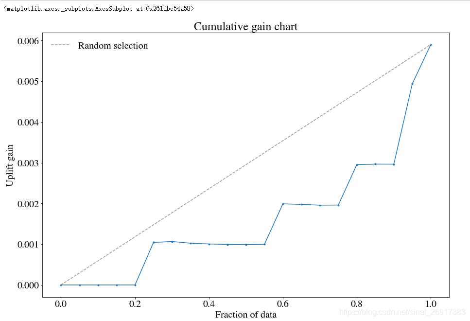 

好的曲线，是均匀分布的；

一个陡峭、不均匀的曲线代表可能存在非常重要的特征，影响着实验组、控制组，需要找到并纠正这样的特征

3.6 通过误差曲线提高模型

绘制误差曲线可以有效地帮助了解预测模型的实际情况。

方法一：up.shuffle_fit实现

通过不断shuffle训练集与验证集，使用相同的超参数，然后把几个模型的结果绘制到同一个qini 图中

up.shuffle_fit(params=up.rand_search_.best_params_, nthread=30, iterations=5) up.plot(show_shuffle_fits=True)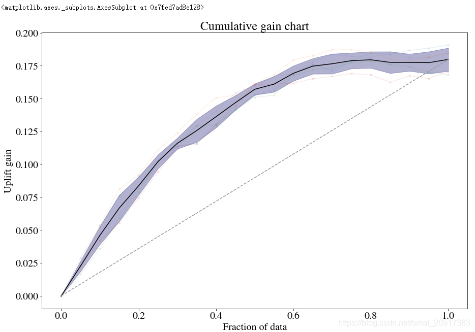 

方法二：up.noise_fit实现
随机扰乱预测集内容，来看会造成如何的误差

up.noise_fit() up.plot(show_noise_fits=True)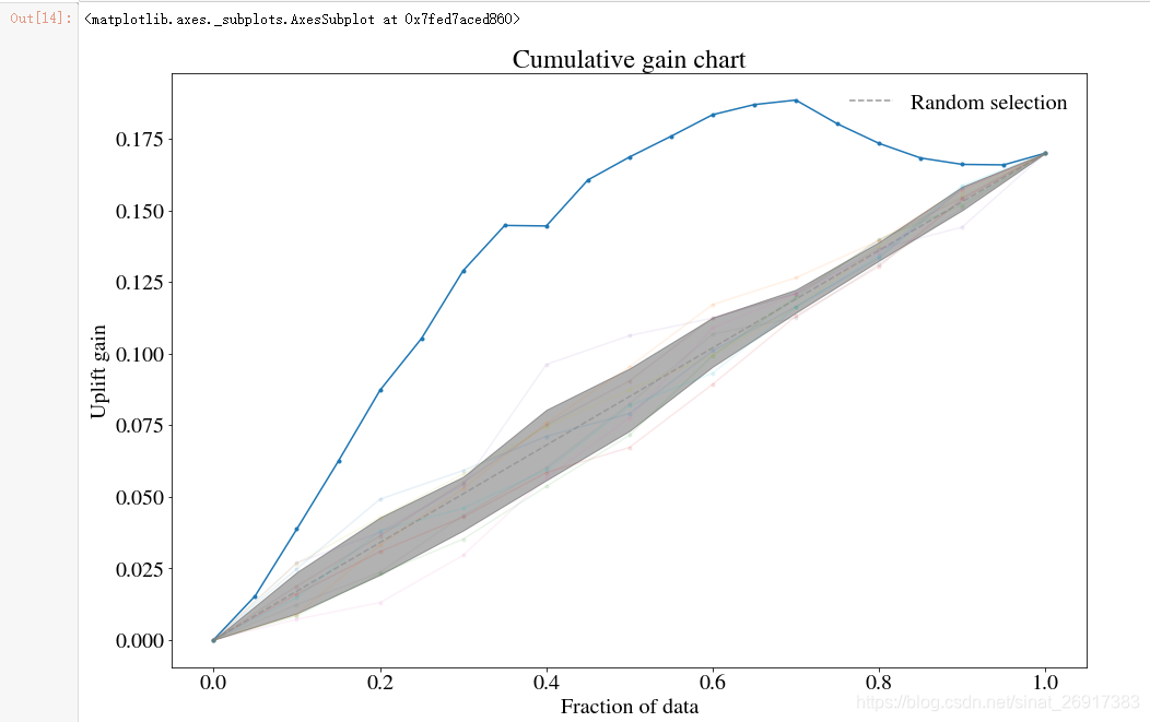 

3.7 用自定义目标函数

特别是对于xgboost，更改目标函数可能会很有用。

例如，如果您喜欢以相等的概率去区分四种人：营销敏感性、反作用人群、自然购买人群、无所谓人群，可以考虑在TransformedOutcome环节使用：MAE

def fair_obj(dtrain, preds): """y = c * abs(x) - c * np.log(abs(abs(x) + c))""" x = preds - dtrain c = 1 den = abs(x) + c treat = dtrain > 0 cont = dtrain < 0 grad = c*x / den hess = c*c / den 2 return grad, hess def huber_approx_obj(dtrain, preds): d = dtrain - preds #remove .get_labels() for sklearn h = 1 #h is delta in the graphic scale = 1 + (d / h) 2 scale_sqrt = np.sqrt(scale) grad = d / scale_sqrt hess = 1 / scale / scale_sqrt return grad, hess def log_cosh_obj(dtrain, preds): x = preds - dtrain grad = np.tanh(x) hess = 1 / np.cosh(x)2 return grad, hess # Specify your dataframe, treatment column, and outcome column. upnew = TransformedOutcome(df, col_treatment='Treatment', col_outcome='Outcome', stratify=df['Treatment'], scoring_method='aqini', scoring_cutoff=0.4) # Using MAE as the objective. from xgboost import XGBRegressor upnew.randomized_search_params['estimator'] = XGBRegressor(objective=log_cosh_obj, nthread=1) upnew.randomized_search(n_iter=10, verbose=3, n_jobs=1) upnew.fit(nthread=50, upnew.rand_search_.best_params_, objective=log_cosh_obj) upnew.plot(label='New objective', n_bins=30)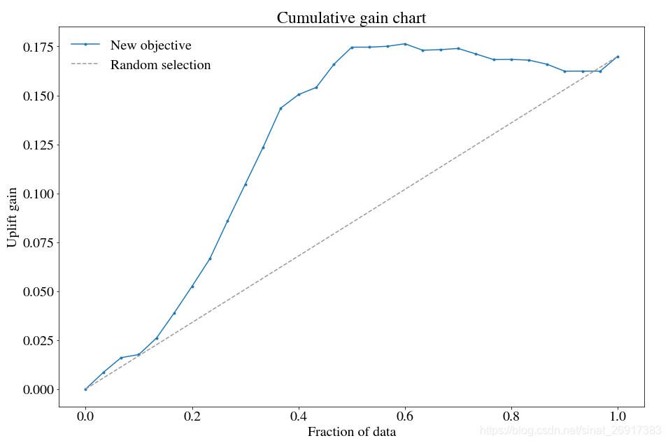 

一般来说，私自调整自定义目标函数效果不好，但是这样的调整行为一定程度纠正：不均衡的处理/控制

3.8 切换不同的模型

from sklearn.tree import DecisionTreeRegressor from sklearn.ensemble import RandomForestRegressor up1 = TransformedOutcome(df, col_treatment='Treatment', col_outcome='Outcome', stratify=df['Treatment'], sklearn_model=RandomForestRegressor) # RandomizedSearchCV. up1.randomized_search(param_distributions={'max_depth': range(1,100), 'min_samples_split': range(1,1000)}, n_iter=10, n_jobs=10) up1.fit(up1.rand_search_.best_params_) up1.plot()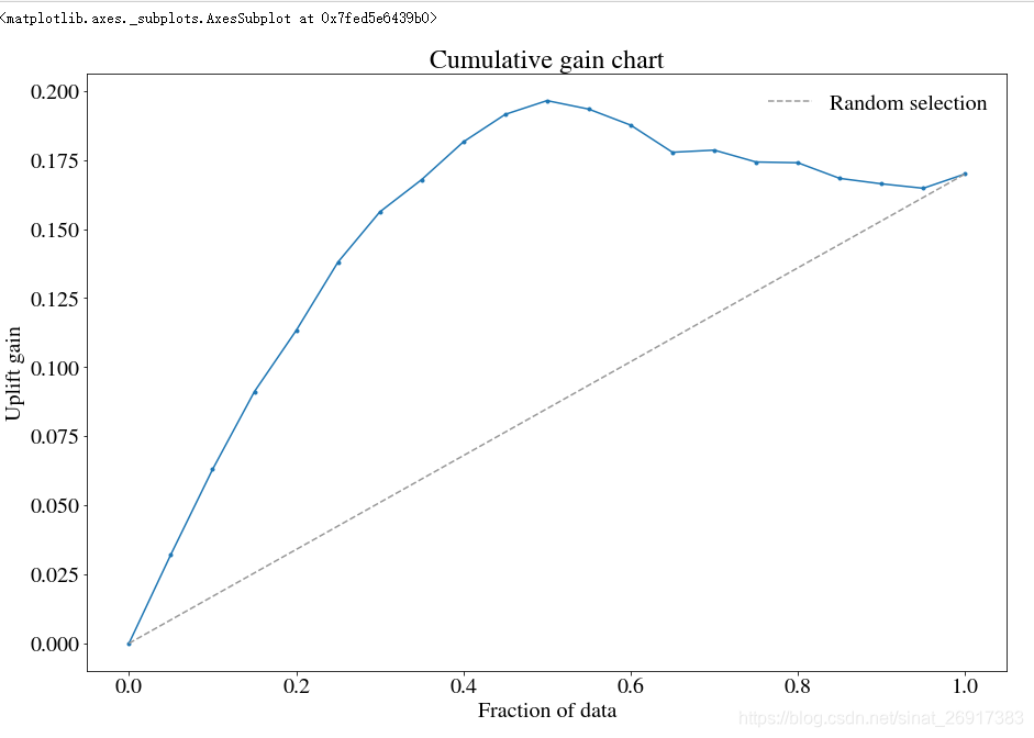 

---

4 案例二：Lalonde_sample

一个完整案例：Lalonde/Lalonde_sample.ipynb

%reload_ext autoreload %autoreload 2 %matplotlib inline import numpy as np, matplotlib as mpl, matplotlib.pyplot as plt, pandas as pd from pylift import TransformedOutcome import pandas as pd pd.options.display.max_rows = 12 #1 载入数据 cols = ['treat', 'age', 'educ', 'black', 'hisp', 'married', 'nodegr','re74','re75','re78'] control_df = pd.read_csv('http://www.nber.org/~rdehejia/data/nswre74_control.txt', sep='\s+', header = None, names = cols) treated_df = pd.read_csv('http://www.nber.org/~rdehejia/data/nswre74_treated.txt', sep='\s+', header = None, names = cols) lalonde_df = pd.concat([control_df, treated_df], ignore_index=True) lalonde_df['u74'] = np.where(lalonde_df['re74'] == 0, 1.0, 0.0) lalonde_df['u75'] = np.where(lalonde_df['re75'] == 0, 1.0, 0.0) #2 清洗数据 df = lalonde_df[['nodegr', 'black', 'hisp', 'age', 'educ', 'married', 'u74', 'u75', 'treat', 're78']].copy() df.rename(columns={'treat':'Treatment', 're78':'Outcome'}, inplace=True) df['Outcome'] = np.where(df['Outcome'] > 0, 1.0, 0.0) # 3 Treatment and Outcome的交叉统计 pd.crosstab(df['Outcome'], df['Treatment'], margins = True) # 4 建模 up = TransformedOutcome(df, col_treatment='Treatment', col_outcome='Outcome', stratify=df['Treatment']) up.randomized_search(n_iter=20, n_jobs=10, random_state=1) up.shuffle_fit(params=up.rand_search_.best_params_, nthread=30, iterations=5) up.plot(show_shuffle_fits=True)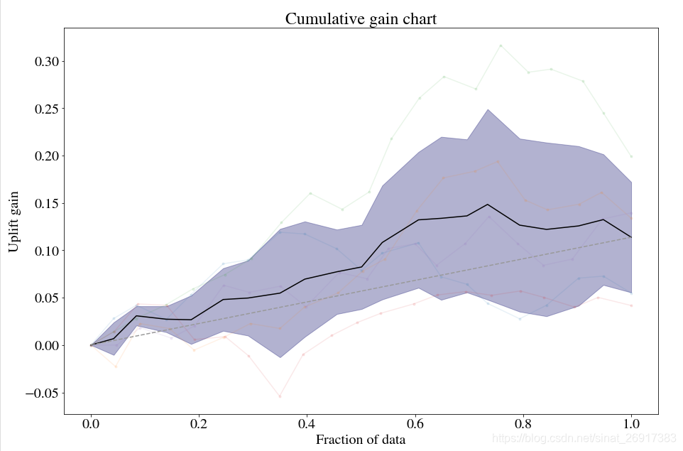 

---

5 pylift 使用介绍

5.1 pylift一些重要属性

一些TransformedOutcome之后，up之中重要属性：

up.randomized_search_params # Parameters that are used in `up.randomized_search()` up.grid_search_params # Parameters that are used in `up.grid_search()` up.transform # Outcome transform function. up.untransform # Reverse of outcome transform function. # Data (`y` in any of these can be replaced with `tc` for treatment or `x`). up.transformed_y_train_pred # The predicted uplift. up.transformed_y_train # The transformed outcome. up.y_train up.y_test up.y # All the `y` data. up.df up.df_train up.df_test # Once a model has been created... up.model up.model_final up.Q_cgains # 'aqini' or 'qini' can be used in place of 'cgains' up.q1_cgains up.q2_cgains 

UpliftEval之后评估曲线信息的重要属性：

upev.PLOTTYPE_x # percentile upev.PLOTTYPE_y 

PLOTTYPE可以用以下任意一种代替：qini，aqini，cgains，cuplift，balance，uplift。由于up.test_results_和up.train_results_是UpliftEval类对象，因此也可以按上面所示类似地对其进行访问。

还可以提取理论上的最大曲线：

# Overfitting theoretical maximal qini curve. upev.qini_max_x # percentile upev.qini_max_y # "Practical" max curve. upev.qini_pmax_x upev.qini_pmax_y # No sleeping dogs curve. upev.qini_nosdmax_x upev.qini_nosdmax_y 

向上
up.train_results_可以用来绘制训练数据上的qini性能

5.2 TransformedOutcome类

参考：Usage: modeling

up = TransformedOutcome(df, col_treatment='Treatment', col_outcome='Converted') 

参数col_treatment是指数据集df中区分是否是treatment group的字段，通过0/1二值区分，
col_outcome相当于label字段，如有转化是1，无转化是0.
其中,stratify参数比较重要，因为其会直接传递给sklearn.model_select .train_test_split用来作为训练集/验证集的拆分

实例化步骤完成了几件事：

• 定义转换函数并转换结果
• 使用train_test_split分割数据
• 设置一个随机状态
• 定义一个untransform函数并使用它来定义一个用于超参数调优的评分函数
• 定义一些默认的超参数。

5.3 up.fit类

RandomizedSearchCV(), GridSearchCV(), 或者Regressor() 都可以传导给： up.randomized_search, up.grid_search, 或者up.fit

up.fit(max_depth=2, nthread=-1) 

举个换模型的例子:

up = TransformedOutcome(df, col_treatment='Test', col_outcome='Converted', sklearn_model=RandomForestRegressor) grid_search_params = { 'estimator': RandomForestRegressor(), 'param_grid': {'min_samples_split': [2,3,5,10,30,100,300,1000,3000,10000]}, 'verbose': True, 'n_jobs': 35, } up.grid_search(grid_search_params) 

5.4 模型保存

跟sklearn一样，self.model_final.to_pickle(PATH)

---

参考文献
1 【营销增益模型实战-Uplift Model原理及应用】
2 Pylift: A Fast Python Package for Uplift Modeling

今天的文章 智能营销增益（Uplift Modeling）模型——pylift库的使用（二）分享到此就结束了，感谢您的阅读。