前言
通过学习前面几个模块,我们已经发现了基于多组学数据找出的乳腺癌各亚型间具有非常显著的分子差异,而我们如果想深入挖掘其背后机制,就需要找出差异表达的基因是哪些,以及这些基因具有什么样的功能。而MOVICS第三个模块,也就是最后一个模块,将会帮助我们实现这个目的。
这一模块的内容需要有一定生物学背景知识才能较好的理解,大家可以通过生信往期的一些推文来进行学习。
主要函数
这一部分的函数主要是行驶差异分析以及富集分析的功能,MOVICS内置了多种常用分析的函数,大家使用时可以根据需要进行选择。
runDEA(): run differential expression analysis with three popular methods for choosing, including edgeR, DESeq2, and limma runMarker(): run biomarker identification to determine uniquely and significantly differential expressed genes for each subtype
runGSEA(): run gene set enrichment analysis (GSEA), calculate activity of functional pathways and generate a pathway-specific heatmap
runGSVA(): run gene set variation analysis to calculate enrichment score of each sample based on given gene set list of interest
runNTP(): run nearest template prediction based on identified biomarkers to evaluate subtypes in external cohorts
runPAM(): run partition around medoids classifier based on discovery cohort to predict subtypes in external cohorts
runKappa(): run consistency evaluation using Kappa statistics between two appraisements that identify or predict current subtypes
代码演示
下面Immugent将进行实操演示:
# run DEA with edgeR
runDEA(dea.method = "edger",
       expr       = count, # raw count data
       moic.res   = cmoic.brca,
       prefix     = "TCGA-BRCA") # prefix of figure name
#> --all samples matched.
#> --you choose edger and please make sure an RNA-Seq count data was provided.
#> edger of CS1_vs_Others done...
#> edger of CS2_vs_Others done...
#> edger of CS3_vs_Others done...
#> edger of CS4_vs_Others done...
#> edger of CS5_vs_Others done...

# run DEA with DESeq2
runDEA(dea.method = "deseq2",
       expr       = count,
       moic.res   = cmoic.brca,
       prefix     = "TCGA-BRCA")
#> --all samples matched.
#> --you choose deseq2 and please make sure an RNA-Seq count data was provided.
#> deseq2 of CS1_vs_Others done...
#> deseq2 of CS2_vs_Others done...
#> deseq2 of CS3_vs_Others done...
#> deseq2 of CS4_vs_Others done...
#> deseq2 of CS5_vs_Others done...

# run DEA with limma
runDEA(dea.method = "limma",
       expr       = fpkm, # normalized expression data
       moic.res   = cmoic.brca,
       prefix     = "TCGA-BRCA")
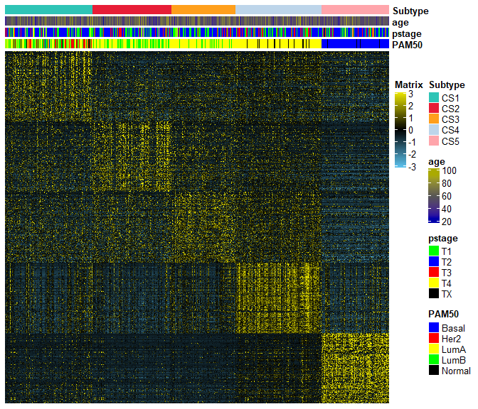
算出差异基因后,做个热图来看一下。
# choose edgeR result to identify subtype-specific up-regulated biomarkers
marker.up <- runMarker(moic.res      = cmoic.brca,
                       dea.method    = "edger", # name of DEA method
                       prefix        = "TCGA-BRCA", # MUST be the same of argument in runDEA()
                       dat.path      = getwd(), # path of DEA files
                       res.path      = getwd(), # path to save marker files
                       p.cutoff      = 0.05, # p cutoff to identify significant DEGs
                       p.adj.cutoff  = 0.05, # padj cutoff to identify significant DEGs
                       dirct         = "up", # direction of dysregulation in expression
                       n.marker      = 100, # number of biomarkers for each subtype
                       doplot        = TRUE, # generate diagonal heatmap
                       norm.expr     = fpkm, # use normalized expression as heatmap input
                       annCol        = annCol, # sample annotation in heatmap
                       annColors     = annColors, # colors for sample annotation
                       show_rownames = FALSE, # show no rownames (biomarker name)
                       fig.name      = "UPREGULATED BIOMARKER HEATMAP")
# MUST locate ABSOLUTE path of msigdb file
MSIGDB.FILE <- system.file("extdata", "c5.bp.v7.1.symbols.xls", package = "MOVICS", mustWork = TRUE)

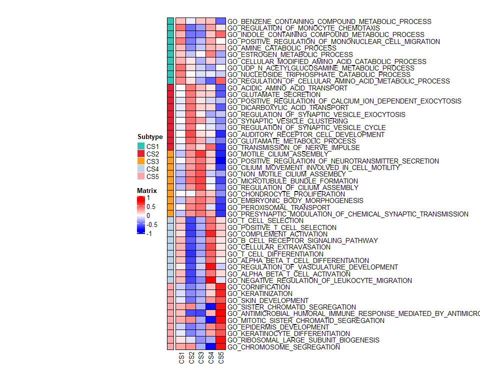
# run GSEA to identify up-regulated GO pathways using results from edgeR
gsea.up <- runGSEA(moic.res     = cmoic.brca,
                   dea.method   = "edger", # name of DEA method
                   prefix       = "TCGA-BRCA", # MUST be the same of argument in runDEA()
                   dat.path     = getwd(), # path of DEA files
                   res.path     = getwd(), # path to save GSEA files
                   msigdb.path  = MSIGDB.FILE, # MUST be the ABSOLUTE path of msigdb file
                   norm.expr    = fpkm, # use normalized expression to calculate enrichment score
                   dirct        = "up", # direction of dysregulation in pathway
                   p.cutoff     = 0.05, # p cutoff to identify significant pathways
                   p.adj.cutoff = 0.25, # padj cutoff to identify significant pathways
                   gsva.method  = "gsva", # method to calculate single sample enrichment score
                   norm.method  = "mean", # normalization method to calculate subtype-specific enrichment score
                   fig.name     = "UPREGULATED PATHWAY HEATMAP")
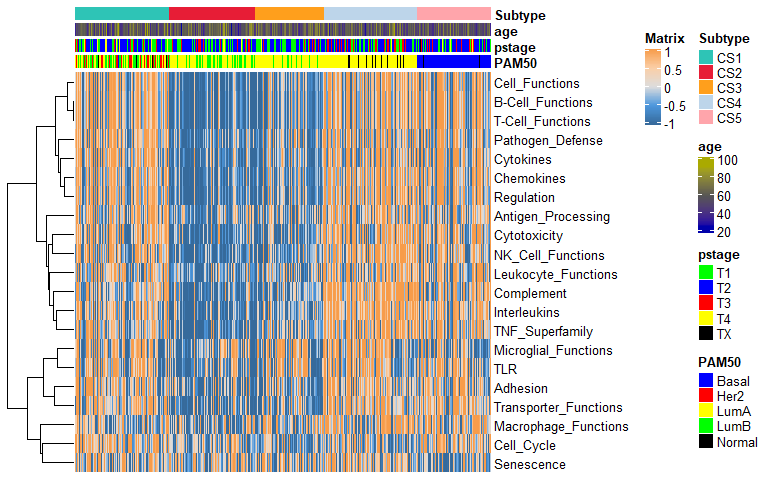
除了GSEA分析还能进行GSVA分析。
# MUST locate ABSOLUTE path of gene set file
GSET.FILE <-
  system.file("extdata", "gene sets of interest.gmt", package = "MOVICS", mustWork = TRUE)
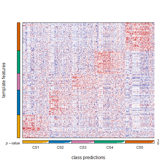
# run NTP in Yau cohort by using up-regulated biomarkers
yau.ntp.pred <- runNTP(expr       = brca.yau$mRNA.expr,
                       templates  = marker.up$templates, # the template has been already prepared in runMarker()
                       scaleFlag  = TRUE, # scale input data (by default)
                       centerFlag = TRUE, # center input data (by default)
                       doPlot     = TRUE, # to generate heatmap
                       fig.name   = "NTP HEATMAP FOR YAU")
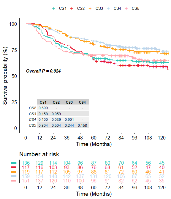
# compare survival outcome in Yau cohort
surv.yau <- compSurv(moic.res         = yau.ntp.pred,
                     surv.info        = brca.yau$clin.info,
                     convt.time       = "m", # switch to month
                     surv.median.line = "hv", # switch to both
                     fig.name         = "KAPLAN-MEIER CURVE OF NTP FOR YAU")
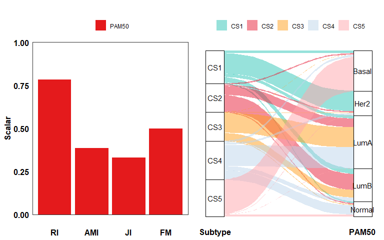
# compare agreement in Yau cohort
agree.yau <- compAgree(moic.res  = yau.ntp.pred,
                       subt2comp = brca.yau$clin.info[, "PAM50", drop = FALSE],
                       doPlot    = TRUE,
                       fig.name  = "YAU PREDICTEDMOIC WITH PAM50")
除了NTP之外,MOVICS还提供了另一种无模型方法来预测亚型。具体来说,runPAM()首先在发现训练集(即TCGA-BRCA)中对medoids (PAM)分类器进行分区训练,以预测外部验证测试集(即BRCA-Yau)中患者的亚型,验证队列中的每个样本被分配到一个子类型标签,其质心与样本的皮尔逊相关性最高。最后,将执行组内比例(IGP)统计来评估发现队列和验证队列之间获得的亚型的相似性和重现性。
yau.pam.pred <- runPAM(train.expr  = fpkm,
                       moic.res    = cmoic.brca,
                       test.expr   = brca.yau$mRNA.expr)

# predict subtype in discovery cohort using NTP
tcga.ntp.pred <- runNTP(expr      = fpkm,
                        templates = marker.up$templates,
                        doPlot    = FALSE)
#> --original template has 500 biomarkers and 500 are matched in external expression profile.
#> cosine correlation distance
#> 643 samples; 5 classes; 100-100 features/class
#> serial processing; 1000 permutation(s)...
#> predicted samples/class (FDR<0.05)
#>
#>  CS1  CS2  CS3  CS4  CS5 <NA>
#>   99  105  138  155  107   39

# predict subtype in discovery cohort using PAM
tcga.pam.pred <- runPAM(train.expr  = fpkm,
                        moic.res    = cmoic.brca,
                        test.expr   = fpkm)
#> --all samples matched.
#> --a total of 13771 genes shared and used.
#> --log2 transformation done for training expression data.
#> --log2 transformation done for testing expression data.

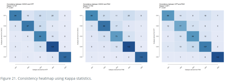
# check consistency between current and NTP-predicted subtype in discovery TCGA-BRCA
runKappa(subt1     = cmoic.brca$clust.res$clust,
         subt2     = tcga.ntp.pred$clust.res$clust,
         subt1.lab = "CMOIC",
         subt2.lab = "NTP",
         fig.name  = "CONSISTENCY HEATMAP FOR TCGA between CMOIC and NTP")

# check consistency between current and PAM-predicted subtype in discovery TCGA-BRCA
runKappa(subt1     = cmoic.brca$clust.res$clust,
         subt2     = tcga.pam.pred$clust.res$clust,
         subt1.lab = "CMOIC",
         subt2.lab = "PAM",
         fig.name  = "CONSISTENCY HEATMAP FOR TCGA between CMOIC and PAM")

# check consistency between NTP and PAM-predicted subtype in validation Yau-BRCA
runKappa(subt1     = yau.ntp.pred$clust.res$clust,
         subt2     = yau.pam.pred$clust.res$clust,
         subt1.lab = "NTP",
         subt2.lab = "PAM",
         fig.name  = "CONSISTENCY HEATMAP FOR YAU")
总结
截止到这篇推文,有关MOVICS包的所有实操部分内容都已结束,本来对这个R包的所有介绍内容都应该完结了。
但是Immugent本着对粉丝极度负责任的态度,后续专门会解读一篇完全依靠这个R包来分析的SCI文章,直到教会大家如何使用MOVICS包分析自己的数据为止,敬请期待!
今天的文章MOVICS系列教程(三) RUN Module分享到此就结束了,感谢您的阅读。
版权声明:本文内容由互联网用户自发贡献,该文观点仅代表作者本人。本站仅提供信息存储空间服务,不拥有所有权,不承担相关法律责任。如发现本站有涉嫌侵权/违法违规的内容, 请发送邮件至 举报,一经查实,本站将立刻删除。
如需转载请保留出处:https://bianchenghao.cn/62362.html

